Chapter 6 Quality Control
6.1 Motivation
Low-quality libraries in scRNA-seq data can arise from a variety of sources such as cell damage during dissociation or failure in library preparation (e.g., inefficient reverse transcription or PCR amplification). These usually manifest as “cells” with low total counts, few expressed genes and high mitochondrial or spike-in proportions. These low-quality libraries are problematic as they can contribute to misleading results in downstream analyses:
- They form their own distinct cluster(s), complicating interpretation of the results. This is most obviously driven by increased mitochondrial proportions or enrichment for nuclear RNAs after cell damage. In the worst case, low-quality libraries generated from different cell types can cluster together based on similarities in the damage-induced expression profiles, creating artificial intermediate states or trajectories between otherwise distinct subpopulations. Additionally, very small libraries can form their own clusters due to shifts in the mean upon transformation (A. Lun 2018).
- They distort the characterization of population heterogeneity during variance estimation or principal components analysis. The first few principal components will capture differences in quality rather than biology, reducing the effectiveness of dimensionality reduction. Similarly, genes with the largest variances will be driven by differences between low- and high-quality cells. The most obvious example involves low-quality libraries with very low counts where scaling normalization inflates the apparent variance of genes that happen to have a non-zero count in those libraries.
- They contain genes that appear to be strongly “upregulated” due to aggressive scaling to normalize for small library sizes. This is most problematic for contaminating transcripts (e.g., from the ambient solution) that are present in all libraries at low but constant levels. Increased scaling in low-quality libraries transforms small counts for these transcripts in large normalized expression values, resulting in apparent upregulation compared to other cells. This can be misleading as the affected genes are often biologically sensible but are actually expressed in another subpopulation.
To avoid - or at least mitigate - these problems, we need to remove these cells at the start of the analysis. This step is commonly referred to as quality control (QC) on the cells. (We will use “library” and “cell” rather interchangeably here, though the distinction will become important when dealing with droplet-based data.) We will demonstrate using a small scRNA-seq dataset from A. T. L. Lun et al. (2017), which is provided with no prior QC so that we can apply our own procedures.
## class: SingleCellExperiment
## dim: 46604 192
## metadata(0):
## assays(1): counts
## rownames(46604): ENSMUSG00000102693 ENSMUSG00000064842 ...
##   ENSMUSG00000095742 CBFB-MYH11-mcherry
## rowData names(1): Length
## colnames(192): SLX-9555.N701_S502.C89V9ANXX.s_1.r_1
##   SLX-9555.N701_S503.C89V9ANXX.s_1.r_1 ...
##   SLX-11312.N712_S508.H5H5YBBXX.s_8.r_1
##   SLX-11312.N712_S517.H5H5YBBXX.s_8.r_1
## colData names(9): Source Name cell line ... spike-in addition block
## reducedDimNames(0):
## altExpNames(2): ERCC SIRV
6.2 Choice of QC metrics
We use several common QC metrics to identify low-quality cells based on their expression profiles. These metrics are described below in terms of reads for SMART-seq2 data, but the same definitions apply to UMI data generated by other technologies like MARS-seq and droplet-based protocols.
- The library size is defined as the total sum of counts across all relevant features for each cell. Here, we will consider the relevant features to be the endogenous genes. Cells with small library sizes are of low quality as the RNA has been lost at some point during library preparation, either due to cell lysis or inefficient cDNA capture and amplification.
- The number of expressed features in each cell is defined as the number of endogenous genes with non-zero counts for that cell. Any cell with very few expressed genes is likely to be of poor quality as the diverse transcript population has not been successfully captured.
- The proportion of reads mapped to spike-in transcripts is calculated relative to the total count across all features (including spike-ins) for each cell. As the same amount of spike-in RNA should have been added to each cell, any enrichment in spike-in counts is symptomatic of loss of endogenous RNA. Thus, high proportions are indicative of poor-quality cells where endogenous RNA has been lost due to, e.g., partial cell lysis or RNA degradation during dissociation.
- In the absence of spike-in transcripts, the proportion of reads mapped to genes in the mitochondrial genome can be used. High proportions are indicative of poor-quality cells (Islam et al. 2014; Ilicic et al. 2016), presumably because of loss of cytoplasmic RNA from perforated cells. The reasoning is that, in the presence of modest damage, the holes in the cell membrane permit efflux of individual transcript molecules but are too small to allow mitochondria to escape, leading to a relative enrichment of mitochondrial transcripts. For single-nuclei RNA-seq experiments, high proportions are also useful as they can mark cells where the cytoplasm has not been successfully stripped.
For each cell, we calculate these QC metrics using the perCellQCMetrics() function from the scater package (McCarthy et al. 2017).
The sum column contains the total count for each cell and the detected column contains the number of detected genes.
The subsets_Mito_percent column contains the percentage of reads mapped to mitochondrial transcripts.
(For demonstration purposes, we show two different approaches of determining the genomic location of each transcript.)
Finally, the altexps_ERCC_percent column contains the percentage of reads mapped to ERCC transcripts.
# Retrieving the mitochondrial transcripts using genomic locations included in
# the row-level annotation for the SingleCellExperiment.
location <- rowRanges(sce.416b)
is.mito <- any(seqnames(location)=="MT")

# ALTERNATIVELY: using resources in AnnotationHub to retrieve chromosomal
# locations given the Ensembl IDs; this should yield the same result.
library(AnnotationHub)
ens.mm.v97 <- AnnotationHub()[["AH73905"]]
chr.loc <- mapIds(ens.mm.v97, keys=rownames(sce.416b),
    keytype="GENEID", column="SEQNAME")
is.mito.alt <- which(chr.loc=="MT")

library(scater)
df <- perCellQCMetrics(sce.416b, subsets=list(Mito=is.mito))
df
## DataFrame with 192 rows and 12 columns
## sum detected subsets_Mito_sum
## <numeric> <numeric> <numeric>
## SLX-9555.N701_S502.C89V9ANXX.s_1.r_1 865936 7618 78790
## SLX-9555.N701_S503.C89V9ANXX.s_1.r_1 1076277 7521 98613
## SLX-9555.N701_S504.C89V9ANXX.s_1.r_1 1180138 8306 100341
## SLX-9555.N701_S505.C89V9ANXX.s_1.r_1 1342593 8143 104882
## SLX-9555.N701_S506.C89V9ANXX.s_1.r_1 1668311 7154 129559
## ... ... ... ...
## SLX-11312.N712_S505.H5H5YBBXX.s_8.r_1 776622 8174 48126
## SLX-11312.N712_S506.H5H5YBBXX.s_8.r_1 1299950 8956 112225
## SLX-11312.N712_S507.H5H5YBBXX.s_8.r_1 1800696 9530 135693
## SLX-11312.N712_S508.H5H5YBBXX.s_8.r_1 46731 6649 3505
## SLX-11312.N712_S517.H5H5YBBXX.s_8.r_1 1866692 10964 150375
## subsets_Mito_detected
## <numeric>
## SLX-9555.N701_S502.C89V9ANXX.s_1.r_1 20
## SLX-9555.N701_S503.C89V9ANXX.s_1.r_1 20
## SLX-9555.N701_S504.C89V9ANXX.s_1.r_1 19
## SLX-9555.N701_S505.C89V9ANXX.s_1.r_1 20
## SLX-9555.N701_S506.C89V9ANXX.s_1.r_1 22
## ... ...
## SLX-11312.N712_S505.H5H5YBBXX.s_8.r_1 20
## SLX-11312.N712_S506.H5H5YBBXX.s_8.r_1 25
## SLX-11312.N712_S507.H5H5YBBXX.s_8.r_1 23
## SLX-11312.N712_S508.H5H5YBBXX.s_8.r_1 16
## SLX-11312.N712_S517.H5H5YBBXX.s_8.r_1 29
## subsets_Mito_percent altexps_ERCC_sum
## <numeric> <numeric>
## SLX-9555.N701_S502.C89V9ANXX.s_1.r_1 9.09882 65278
## SLX-9555.N701_S503.C89V9ANXX.s_1.r_1 9.16242 74748
## SLX-9555.N701_S504.C89V9ANXX.s_1.r_1 8.50248 60878
## SLX-9555.N701_S505.C89V9ANXX.s_1.r_1 7.81190 60073
## SLX-9555.N701_S506.C89V9ANXX.s_1.r_1 7.76588 136810
## ... ... ...
## SLX-11312.N712_S505.H5H5YBBXX.s_8.r_1 6.19684 61575
## SLX-11312.N712_S506.H5H5YBBXX.s_8.r_1 8.63302 94982
## SLX-11312.N712_S507.H5H5YBBXX.s_8.r_1 7.53559 113707
## SLX-11312.N712_S508.H5H5YBBXX.s_8.r_1 7.50037 7580
## SLX-11312.N712_S517.H5H5YBBXX.s_8.r_1 8.05569 48664
## altexps_ERCC_detected
## <numeric>
## SLX-9555.N701_S502.C89V9ANXX.s_1.r_1 39
## SLX-9555.N701_S503.C89V9ANXX.s_1.r_1 40
## SLX-9555.N701_S504.C89V9ANXX.s_1.r_1 42
## SLX-9555.N701_S505.C89V9ANXX.s_1.r_1 42
## SLX-9555.N701_S506.C89V9ANXX.s_1.r_1 44
## ... ...
## SLX-11312.N712_S505.H5H5YBBXX.s_8.r_1 39
## SLX-11312.N712_S506.H5H5YBBXX.s_8.r_1 41
## SLX-11312.N712_S507.H5H5YBBXX.s_8.r_1 40
## SLX-11312.N712_S508.H5H5YBBXX.s_8.r_1 44
## SLX-11312.N712_S517.H5H5YBBXX.s_8.r_1 39
## altexps_ERCC_percent altexps_SIRV_sum
## <numeric> <numeric>
## SLX-9555.N701_S502.C89V9ANXX.s_1.r_1 6.80658 27828
## SLX-9555.N701_S503.C89V9ANXX.s_1.r_1 6.28030 39173
## SLX-9555.N701_S504.C89V9ANXX.s_1.r_1 4.78949 30058
## SLX-9555.N701_S505.C89V9ANXX.s_1.r_1 4.18567 32542
## SLX-9555.N701_S506.C89V9ANXX.s_1.r_1 7.28887 71850
## ... ... ...
## SLX-11312.N712_S505.H5H5YBBXX.s_8.r_1 7.17620 19848
## SLX-11312.N712_S506.H5H5YBBXX.s_8.r_1 6.65764 31729
## SLX-11312.N712_S507.H5H5YBBXX.s_8.r_1 5.81467 41116
## SLX-11312.N712_S508.H5H5YBBXX.s_8.r_1 13.48898 1883
## SLX-11312.N712_S517.H5H5YBBXX.s_8.r_1 2.51930 16289
## altexps_SIRV_detected
## <numeric>
## SLX-9555.N701_S502.C89V9ANXX.s_1.r_1 7
## SLX-9555.N701_S503.C89V9ANXX.s_1.r_1 7
## SLX-9555.N701_S504.C89V9ANXX.s_1.r_1 7
## SLX-9555.N701_S505.C89V9ANXX.s_1.r_1 7
## SLX-9555.N701_S506.C89V9ANXX.s_1.r_1 7
## ... ...
## SLX-11312.N712_S505.H5H5YBBXX.s_8.r_1 7
## SLX-11312.N712_S506.H5H5YBBXX.s_8.r_1 7
## SLX-11312.N712_S507.H5H5YBBXX.s_8.r_1 7
## SLX-11312.N712_S508.H5H5YBBXX.s_8.r_1 7
## SLX-11312.N712_S517.H5H5YBBXX.s_8.r_1 7
## altexps_SIRV_percent total
## <numeric> <numeric>
## SLX-9555.N701_S502.C89V9ANXX.s_1.r_1 2.90165 959042
## SLX-9555.N701_S503.C89V9ANXX.s_1.r_1 3.29130 1190198
## SLX-9555.N701_S504.C89V9ANXX.s_1.r_1 2.36477 1271074
## SLX-9555.N701_S505.C89V9ANXX.s_1.r_1 2.26741 1435208
## SLX-9555.N701_S506.C89V9ANXX.s_1.r_1 3.82798 1876971
## ... ... ...
## SLX-11312.N712_S505.H5H5YBBXX.s_8.r_1 2.313165 858045
## SLX-11312.N712_S506.H5H5YBBXX.s_8.r_1 2.224004 1426661
## SLX-11312.N712_S507.H5H5YBBXX.s_8.r_1 2.102562 1955519
## SLX-11312.N712_S508.H5H5YBBXX.s_8.r_1 3.350892 56194
## SLX-11312.N712_S517.H5H5YBBXX.s_8.r_1 0.843271 1931645Alternatively, users may prefer to use the addPerCellQC() function.
This computes and appends the per-cell QC statistics to the colData of the SingleCellExperiment object,
allowing us to retain all relevant information in a single object for later manipulation.
##  [1] "Source Name"              "cell line"
##  [3] "cell type"                "single cell well quality"
##  [5] "genotype"                 "phenotype"
##  [7] "strain"                   "spike-in addition"
##  [9] "block"                    "sum"
## [11] "detected"                 "subsets_Mito_sum"
## [13] "subsets_Mito_detected"    "subsets_Mito_percent"
## [15] "altexps_ERCC_sum"         "altexps_ERCC_detected"
## [17] "altexps_ERCC_percent"     "altexps_SIRV_sum"
## [19] "altexps_SIRV_detected"    "altexps_SIRV_percent"
## [21] "total"
A key assumption here is that the QC metrics are independent of the biological state of each cell. Poor values (e.g., low library sizes, high mitochondrial proportions) are presumed to be driven by technical factors rather than biological processes, meaning that the subsequent removal of cells will not misrepresent the biology in downstream analyses. Major violations of this assumption would potentially result in the loss of cell types that have, say, systematically low RNA content or high numbers of mitochondria. We can check for such violations using some diagnostics described in Sections 6.4 and 6.5.
6.3 Identifying low-quality cells
6.3.1 With fixed thresholds
The simplest approach to identifying low-quality cells is to apply thresholds on the QC metrics. For example, we might consider cells to be low quality if they have library sizes below 100,000 reads; express fewer than 5,000 genes; have spike-in proportions above 10%; or have mitochondrial proportions above 10%.
qc.lib <- df$sum < 1e5
qc.nexprs <- df$detected < 5e3
qc.spike <- df$altexps_ERCC_percent > 10
qc.mito <- df$subsets_Mito_percent > 10
discard <- qc.lib | qc.nexprs | qc.spike | qc.mito

# Summarize the number of cells removed for each reason.
DataFrame(LibSize=sum(qc.lib), NExprs=sum(qc.nexprs),
    SpikeProp=sum(qc.spike), MitoProp=sum(qc.mito), Total=sum(discard))
## DataFrame with 1 row and 5 columns
## LibSize NExprs SpikeProp MitoProp Total
## <integer> <integer> <integer> <integer> <integer>
## 1 3 0 19 14 33While simple, this strategy requires considerable experience to determine appropriate thresholds for each experimental protocol and biological system. Thresholds for read count-based data are simply not applicable for UMI-based data, and vice versa. Differences in mitochondrial activity or total RNA content require constant adjustment of the mitochondrial and spike-in thresholds, respectively, for different biological systems. Indeed, even with the same protocol and system, the appropriate threshold can vary from run to run due to the vagaries of cDNA capture efficiency and sequencing depth per cell.
6.3.2 With adaptive thresholds
6.3.2.1 Identifying outliers
To obtain an adaptive threshold, we assume that most of the dataset consists of high-quality cells. We then identify cells that are outliers for the various QC metrics, based on the median absolute deviation (MAD) from the median value of each metric across all cells. Specifically, a value is considered an outlier if it is more than 3 MADs from the median in the “problematic” direction. This is loosely motivated by the fact that such a filter will retain 99% of non-outlier values that follow a normal distribution.
For the 416B data, we identify cells with log-transformed library sizes that are more than 3 MADs below the median.
A log-transformation is used to improve resolution at small values when type="lower".
Specifically, it guarantees that the threshold is not a negative value, which would be meaningless for a non-negative metric.
Furthermore, it is not uncommon for the distribution of library sizes to exhibit a heavy right tail;
the log-transformation avoids inflation of the MAD in a manner that might compromise outlier detection on the left tail.
(More generally, it makes the distribution seem more normal to justify the 99% rationale mentioned above.)
We do the same for the log-transformed number of expressed genes.
isOutlier() will also return the exact filter thresholds for each metric in the attributes of the output vector.
These are useful for checking whether the automatically selected thresholds are appropriate.
##  lower higher
## 434083 Inf## lower higher
## 5231 InfWe identify outliers for the proportion-based metrics with the same function. These distributions frequently exhibit a heavy right tail, but unlike the two previous metrics, it is the right tail itself that contains the putative low-quality cells. Thus, we do not perform any transformation to shrink the tail - rather, our hope is that the cells in the tail are identified as large outliers. (While it is theoretically possible to obtain a meaningless threshold above 100%, this is rare enough to not be of practical concern.)
##  lower higher
## -Inf 14.15## lower higher
## -Inf 11.92A cell that is an outlier for any of these metrics is considered to be of low quality and discarded.
discard2 <- qc.lib2 | qc.nexprs2 | qc.spike2 | qc.mito2

# Summarize the number of cells removed for each reason.
DataFrame(LibSize=sum(qc.lib2), NExprs=sum(qc.nexprs2),
    SpikeProp=sum(qc.spike2), MitoProp=sum(qc.mito2), Total=sum(discard2))
## DataFrame with 1 row and 5 columns
## LibSize NExprs SpikeProp MitoProp Total
## <integer> <integer> <integer> <integer> <integer>
## 1 4 0 1 2 6Alternatively, this entire process can be done in a single step using the quickPerCellQC() function.
This is a wrapper that simply calls isOutlier() with the settings described above.
reasons <- quickPerCellQC(df,
    sub.fields=c("subsets_Mito_percent", "altexps_ERCC_percent"))
colSums(as.matrix(reasons))
## low_lib_size low_n_features high_subsets_Mito_percent
## 4 0 2
## high_altexps_ERCC_percent discard
## 1 6With this strategy, the thresholds adapt to both the location and spread of the distribution of values for a given metric. This allows the QC procedure to adjust to changes in sequencing depth, cDNA capture efficiency, mitochondrial content, etc. without requiring any user intervention or prior experience. However, it does require some implicit assumptions that are discussed below in more detail.
6.3.2.2 Assumptions of outlier detection
Outlier detection assumes that most cells are of acceptable quality. This is usually reasonable and can be experimentally supported in some situations by visually checking that the cells are intact, e.g., on the microwell plate. If most cells are of (unacceptably) low quality, the adaptive thresholds will obviously fail as they cannot remove the majority of cells. Of course, what is acceptable or not is in the eye of the beholder - neurons, for example, are notoriously difficult to dissociate, and we would often retain cells in a neuronal scRNA-seq dataset with QC metrics that would be unacceptable in a more amenable system like embryonic stem cells.
Another assumption mentioned earlier is that the QC metrics are independent of the biological state of each cell. This is most likely to be violated in highly heterogeneous cell populations where some cell types naturally have, e.g., less total RNA (see Figure 3A of Germain, Sonrel, and Robinson (2020)) or more mitochondria. Such cells are more likely to be considered outliers and removed, even in the absence of any technical problems with their capture or sequencing. The use of the MAD mitigates this problem to some extent by accounting for biological variability in the QC metrics. A heterogeneous population should have higher variability in the metrics among high-quality cells, increasing the MAD and reducing the chance of incorrectly removing particular cell types (at the cost of reducing power to remove low-quality cells).
In general, these assumptions are either reasonable or their violations have little effect on downstream conclusions. Nonetheless, it is helpful to keep them in mind when interpreting the results.
6.3.2.3 Considering experimental factors
More complex studies may involve batches of cells generated with different experimental parameters (e.g., sequencing depth). In such cases, the adaptive strategy should be applied to each batch separately. It makes little sense to compute medians and MADs from a mixture distribution containing samples from multiple batches. For example, if the sequencing coverage is lower in one batch compared to the others, it will drag down the median and inflate the MAD. This will reduce the suitability of the adaptive threshold for the other batches.
If each batch is represented by its own SingleCellExperiment, the isOutlier() function can be directly applied to each batch as shown above.
However, if cells from all batches have been merged into a single SingleCellExperiment, the batch= argument should be used to ensure that outliers are identified within each batch.
This allows isOutlier() to accommodate systematic differences in the QC metrics across batches.
We will again illustrate using the 416B dataset, which contains two experimental factors - plate of origin and oncogene induction status.
We combine these factors together and use this in the batch= argument to isOutlier() via quickPerCellQC().
This results in the removal of slightly more cells as the MAD is no longer inflated by (i) systematic differences in sequencing depth between batches and (ii) differences in number of genes expressed upon oncogene induction.
batch <- paste0(sce.416b$phenotype, "-", sce.416b$block)
batch.reasons <- quickPerCellQC(df, batch=batch,
    sub.fields=c("subsets_Mito_percent", "altexps_ERCC_percent"))
colSums(as.matrix(batch.reasons))
## low_lib_size low_n_features high_subsets_Mito_percent
## 5 4 2
## high_altexps_ERCC_percent discard
## 6 9That said, the use of batch= involves the stronger assumption that most cells in each batch are of high quality.
If an entire batch failed, outlier detection will not be able to act as an appropriate QC filter for that batch.
For example, two batches in the Grun et al. (2016) human pancreas dataset contain a substantial proportion of putative damaged cells with higher ERCC content than the other batches (Figure 6.1).
This inflates the median and MAD within those batches, resulting in a failure to remove the assumed low-quality cells.
In such cases, it is better to compute a shared median and MAD from the other batches and use those estimates to obtain an appropriate filter threshold for cells in the problematic batches, as shown below.
library(scRNAseq)
sce.grun <- GrunPancreasData()
sce.grun <- addPerCellQC(sce.grun)

# First attempt with batch-specific thresholds.
discard.ercc <- isOutlier(sce.grun$altexps_ERCC_percent,
    type="higher", batch=sce.grun$donor)
with.blocking <- plotColData(sce.grun, x="donor", y="altexps_ERCC_percent",
    colour_by=I(discard.ercc))

# Second attempt, sharing information across batches
# to avoid dramatically different thresholds for unusual batches.
discard.ercc2 <- isOutlier(sce.grun$altexps_ERCC_percent,
    type="higher", batch=sce.grun$donor,
    subset=sce.grun$donor %in% c("D17", "D2", "D7"))
without.blocking <- plotColData(sce.grun, x="donor", y="altexps_ERCC_percent",
    colour_by=I(discard.ercc2))

gridExtra::grid.arrange(with.blocking, without.blocking, ncol=2)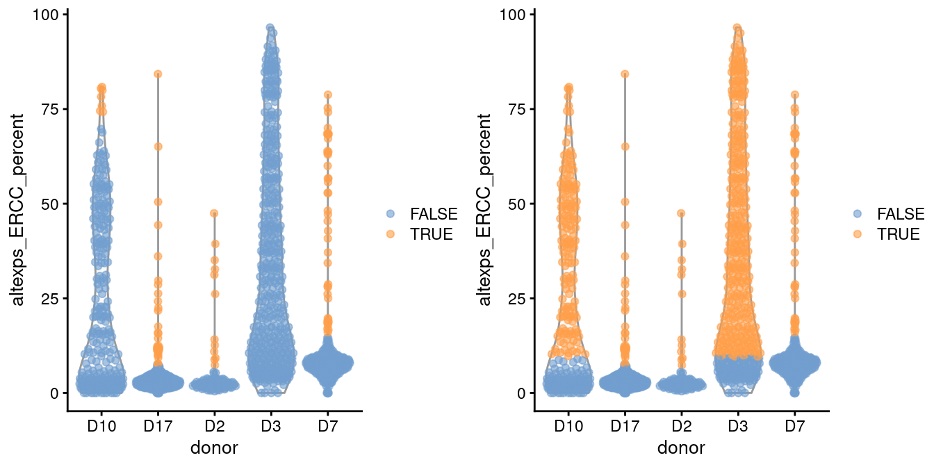
Figure 6.1: Distribution of the proportion of ERCC transcripts in each donor of the Grun pancreas dataset. Each point represents a cell and is coloured according to whether it was identified as an outlier within each batch (left) or using a common threshold (right).
To identify problematic batches, one useful rule of thumb is to find batches with QC thresholds that are themselves outliers compared to the thresholds of other batches. The assumption here is that most batches consist of a majority of high quality cells such that the threshold value should follow some unimodal distribution across “typical” batches. If we observe a batch with an extreme threshold value, we may suspect that it contains a large number of low-quality cells that inflate the per-batch MAD. We demonstrate this process below for the Grun et al. (2016) data.
##     D10     D17      D2      D3      D7
## 73.611 7.600 6.011 113.106 15.217## [1] "D10" "D3"If we cannot assume that most batches contain a majority of high-quality cells, then all bets are off; we must revert to the approach of picking an arbitrary threshold value (Section 6.3.1) and hoping for the best.
6.3.3 Other approaches
Another strategy is to identify outliers in high-dimensional space based on the QC metrics for each cell.
We use methods from robustbase to quantify the “outlyingness” of each cells based on their QC metrics, and then use isOutlier() to identify low-quality cells that exhibit unusually high levels of outlyingness.
stats <- cbind(log10(df$sum), log10(df$detected),
    df$subsets_Mito_percent, df$altexps_ERCC_percent)

library(robustbase)
outlying <- adjOutlyingness(stats, only.outlyingness = TRUE)
multi.outlier <- isOutlier(outlying, type = "higher")
summary(multi.outlier)
## Mode FALSE TRUE
## logical 183 9This and related approaches like PCA-based outlier detection and support vector machines can provide more power to distinguish low-quality cells from high-quality counterparts (Ilicic et al. 2016) as they can exploit patterns across many QC metrics. However, this comes at some cost to interpretability, as the reason for removing a given cell may not always be obvious.
For completeness, we note that outliers can also be identified from the gene expression profiles, rather than QC metrics. We consider this to be a risky strategy as it can remove high-quality cells in rare populations.
6.4 Checking diagnostic plots
It is good practice to inspect the distributions of QC metrics (Figure 6.2) to identify possible problems. In the most ideal case, we would see normal distributions that would justify the 3 MAD threshold used in outlier detection. A large proportion of cells in another mode suggests that the QC metrics might be correlated with some biological state, potentially leading to the loss of distinct cell types during filtering; or that there were inconsistencies with library preparation for a subset of cells, a not-uncommon phenomenon in plate-based protocols. Batches with systematically poor values for any metric can then be quickly identified for further troubleshooting or outright removal, much like in Figure 6.1 above.
colData(sce.416b) <- cbind(colData(sce.416b), df)
sce.416b$block <- factor(sce.416b$block)
sce.416b$phenotype <- ifelse(grepl("induced", sce.416b$phenotype),
    "induced", "wild type")
sce.416b$discard <- reasons$discard

gridExtra::grid.arrange(
    plotColData(sce.416b, x="block", y="sum", colour_by="discard",
        other_fields="phenotype") + facet_wrap(~phenotype) +
        scale_y_log10() + ggtitle("Total count"),
    plotColData(sce.416b, x="block", y="detected", colour_by="discard",
        other_fields="phenotype") + facet_wrap(~phenotype) +
        scale_y_log10() + ggtitle("Detected features"),
    plotColData(sce.416b, x="block", y="subsets_Mito_percent",
        colour_by="discard", other_fields="phenotype") +
        facet_wrap(~phenotype) + ggtitle("Mito percent"),
    plotColData(sce.416b, x="block", y="altexps_ERCC_percent",
        colour_by="discard", other_fields="phenotype") +
        facet_wrap(~phenotype) + ggtitle("ERCC percent"),
    ncol=1
)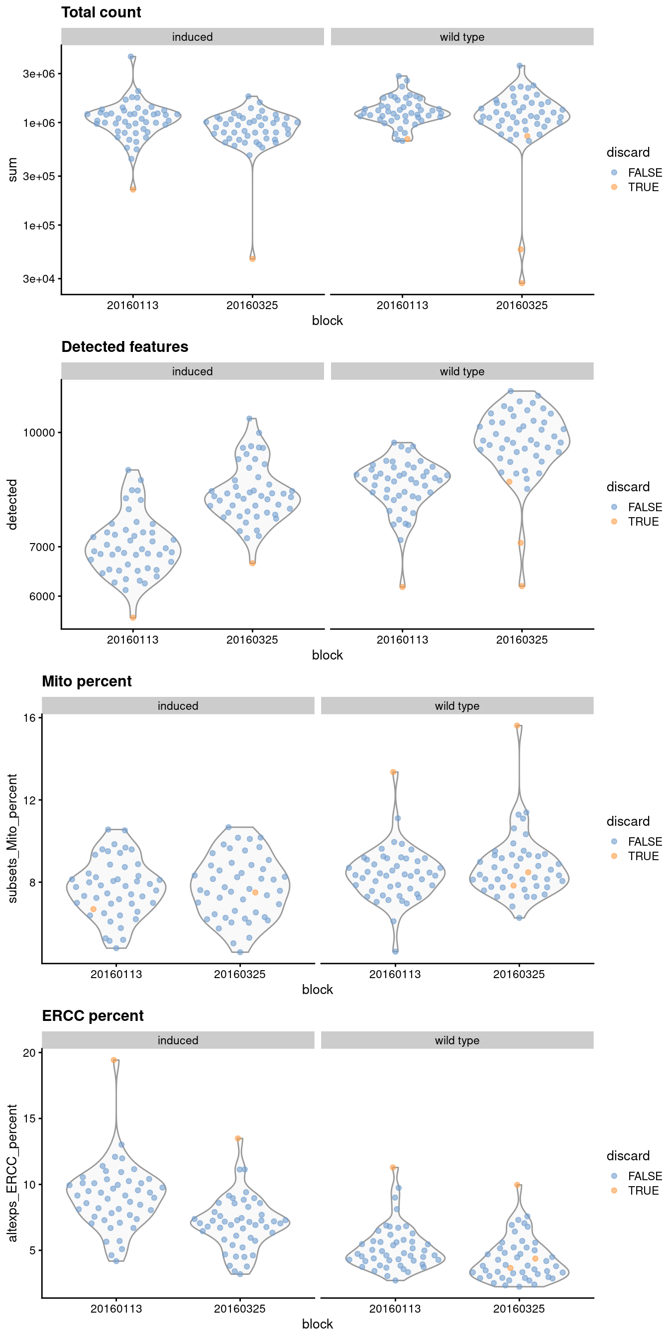
Figure 6.2: Distribution of QC metrics for each batch and phenotype in the 416B dataset. Each point represents a cell and is colored according to whether it was discarded, respectively.
Another useful diagnostic involves plotting the proportion of mitochondrial counts against some of the other QC metrics. The aim is to confirm that there are no cells with both large total counts and large mitochondrial counts, to ensure that we are not inadvertently removing high-quality cells that happen to be highly metabolically active (e.g., hepatocytes). We demonstrate using data from a larger experiment involving the mouse brain (Zeisel et al. 2015); in this case, we do not observe any points in the top-right corner in Figure 6.3 that might potentially correspond to metabolically active, undamaged cells.
#--- loading ---#
library(scRNAseq)
sce.zeisel <- ZeiselBrainData()

library(scater)
sce.zeisel <- aggregateAcrossFeatures(sce.zeisel,
    id=sub("_loc[0-9]+$", "", rownames(sce.zeisel)))

#--- gene-annotation ---#
library(org.Mm.eg.db)
rowData(sce.zeisel)$Ensembl <- mapIds(org.Mm.eg.db,
    keys=rownames(sce.zeisel), keytype="SYMBOL", column="ENSEMBL")
sce.zeisel <- addPerCellQC(sce.zeisel,
subsets=list(Mt=rowData(sce.zeisel)$featureType=="mito"))
qc <- quickPerCellQC(colData(sce.zeisel),
sub.fields=c("altexps_ERCC_percent", "subsets_Mt_percent"))
sce.zeisel$discard <- qc$discard
plotColData(sce.zeisel, x="sum", y="subsets_Mt_percent", colour_by="discard")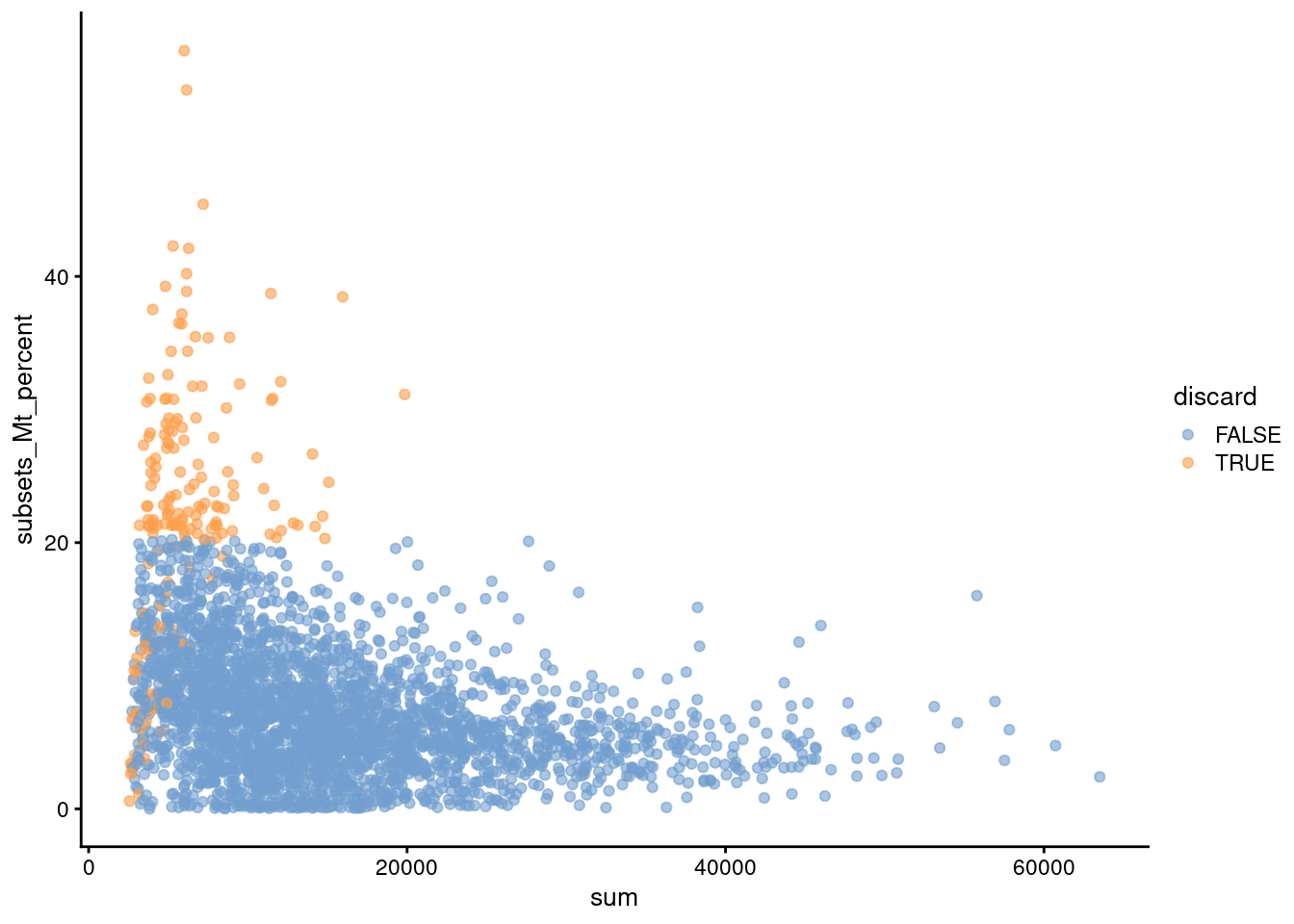
Figure 6.3: Percentage of UMIs assigned to mitochondrial transcripts in the Zeisel brain dataset, plotted against the total number of UMIs (top). Each point represents a cell and is colored according to whether it was considered low-quality and discarded.
Comparison of the ERCC and mitochondrial percentages can also be informative (Figure 6.4). Low-quality cells with small mitochondrial percentages, large spike-in percentages and small library sizes are likely to be stripped nuclei, i.e., they have been so extensively damaged that they have lost all cytoplasmic content. On the other hand, cells with high mitochondrial percentages and low ERCC percentages may represent undamaged cells that are metabolically active. This interpretation also applies for single-nuclei studies but with a switch of focus: the stripped nuclei become the libraries of interest while the undamaged cells are considered to be low quality.
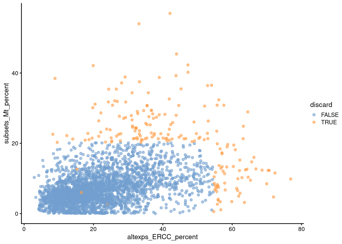
Figure 6.4: Percentage of UMIs assigned to mitochondrial transcripts in the Zeisel brain dataset, plotted against the percentage of UMIs assigned to spike-in transcripts (bottom). Each point represents a cell and is colored according to whether it was considered low-quality and discarded.
We see that all of these metrics exhibit weak correlations to each other, presumably a manifestation of a common underlying effect of cell damage. The weakness of the correlations motivates the use of several metrics to capture different aspects of technical quality. Of course, the flipside is that these metrics may also represent different aspects of biology, increasing the risk of discarding entire cell types as discussed in Section 6.3.2.2.
6.5 Removing low-quality cells
Once low-quality cells have been identified, we can choose to either remove them or mark them.
Removal is the most straightforward option and is achieved by subsetting the SingleCellExperiment by column.
In this case, we use the low-quality calls from Section 6.3.2.3 to generate a subsetted SingleCellExperiment that we would use for downstream analyses.
The biggest practical concern during QC is whether an entire cell type is inadvertently discarded. There is always some risk of this occurring as the QC metrics are never fully independent of biological state. We can diagnose cell type loss by looking for systematic differences in gene expression between the discarded and retained cells. To demonstrate, we compute the average count across the discarded and retained pools in the 416B data set, and we compute the log-fold change between the pool averages.
# Using the 'discard' vector for demonstration purposes,
# as it has more cells for stable calculation of 'lost'.
lost <- calculateAverage(counts(sce.416b)[,!discard])
kept <- calculateAverage(counts(sce.416b)[,discard])

library(edgeR)
logged <- cpm(cbind(lost, kept), log=TRUE, prior.count=2)
logFC <- logged[,1] - logged[,2]
abundance <- rowMeans(logged)
If the discarded pool is enriched for a certain cell type, we should observe increased expression of the corresponding marker genes. No systematic upregulation of genes is apparent in the discarded pool in Figure 6.5, suggesting that the QC step did not inadvertently filter out a cell type in the 416B dataset.
plot(abundance, logFC, xlab="Average count", ylab="Log-FC (lost/kept)", pch=16)
points(abundance[is.mito], logFC[is.mito], col="dodgerblue", pch=16)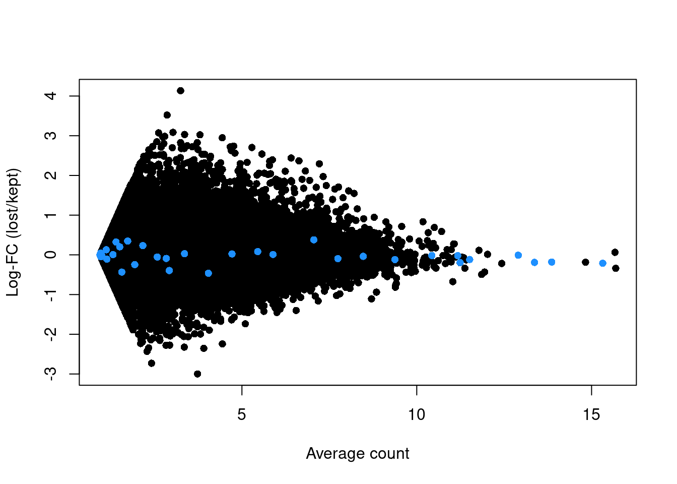
Figure 6.5: Log-fold change in expression in the discarded cells compared to the retained cells in the 416B dataset. Each point represents a gene with mitochondrial transcripts in blue.
For comparison, let us consider the QC step for the PBMC dataset from 10X Genomics (Zheng et al. 2017). We’ll apply an arbitrary fixed threshold on the library size to filter cells rather than using any outlier-based method. Specifically, we remove all libraries with a library size below 500.
#--- loading ---#
library(DropletTestFiles)
raw.path <- getTestFile("tenx-2.1.0-pbmc4k/1.0.0/raw.tar.gz")
out.path <- file.path(tempdir(), "pbmc4k")
untar(raw.path, exdir=out.path)

library(DropletUtils)
fname <- file.path(out.path, "raw_gene_bc_matrices/GRCh38")
sce.pbmc <- read10xCounts(fname, col.names=TRUE)

#--- gene-annotation ---#
library(scater)
rownames(sce.pbmc) <- uniquifyFeatureNames(
    rowData(sce.pbmc)$ID, rowData(sce.pbmc)$Symbol)

library(EnsDb.Hsapiens.v86)
location <- mapIds(EnsDb.Hsapiens.v86, keys=rowData(sce.pbmc)$ID,
    column="SEQNAME", keytype="GENEID")

#--- cell-detection ---#
set.seed(100)
e.out <- emptyDrops(counts(sce.pbmc))
sce.pbmc <- sce.pbmc[,which(e.out$FDR <= 0.001)]
discard <- colSums(counts(sce.pbmc)) < 500
lost <- calculateAverage(counts(sce.pbmc)[,discard])
kept <- calculateAverage(counts(sce.pbmc)[,!discard])
logged <- edgeR::cpm(cbind(lost, kept), log=TRUE, prior.count=2)
logFC <- logged[,1] - logged[,2]
abundance <- rowMeans(logged)The presence of a distinct population in the discarded pool manifests in Figure 6.6 as a set of genes that are strongly upregulated in lost.
This includes PF4, PPBP and SDPR, which (spoiler alert!) indicates that there is a platelet population that has been discarded by alt.discard.
plot(abundance, logFC, xlab="Average count", ylab="Log-FC (lost/kept)", pch=16)
platelet <- c("PF4", "PPBP", "SDPR")
points(abundance[platelet], logFC[platelet], col="orange", pch=16)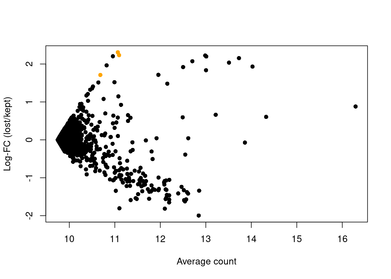
Figure 6.6: Average counts across all discarded and retained cells in the PBMC dataset, after using a more stringent filter on the total UMI count. Each point represents a gene, with platelet-related genes highlighted in orange.
If we suspect that cell types have been incorrectly discarded by our QC procedure, the most direct solution is to relax the QC filters for metrics that are associated with genuine biological differences.
For example, outlier detection can be relaxed by increasing nmads= in the isOutlier() calls.
Of course, this increases the risk of retaining more low-quality cells and encountering the problems discussed in Section 6.1.
The logical endpoint of this line of reasoning is to avoid filtering altogether, as discussed in Section 6.6.
As an aside, it is worth mentioning that the true technical quality of a cell may also be correlated with its type. (This differs from a correlation between the cell type and the QC metrics, as the latter are our imperfect proxies for quality.) This can arise if some cell types are not amenable to dissociation or microfluidics handling during the scRNA-seq protocol. In such cases, it is possible to “correctly” discard an entire cell type during QC if all of its cells are damaged. Indeed, concerns over the computational removal of cell types during QC are probably minor compared to losses in the experimental protocol.
6.6 Marking low-quality cells
The other option is to simply mark the low-quality cells as such and retain them in the downstream analysis. The aim here is to allow clusters of low-quality cells to form, and then to identify and ignore such clusters during interpretation of the results. This approach avoids discarding cell types that have poor values for the QC metrics, giving users an opportunity to decide whether a cluster of such cells represents a genuine biological state.
The downside is that it shifts the burden of QC to the interpretation of the clusters, which is already the bottleneck in scRNA-seq data analysis (Chapters 10, 11 and 12). Indeed, if we do not trust the QC metrics, we would have to distinguish between genuine cell types and low-quality cells based only on marker genes, and this is not always easy due to the tendency of the latter to “express” interesting genes (Section 6.1). Retention of low-quality cells also compromises the accuracy of the variance modelling, requiring, e.g., use of more PCs to offset the fact that the early PCs are driven by differences between low-quality and other cells.
For routine analyses, we suggest performing removal by default to avoid complications from low-quality cells. This allows most of the population structure to be characterized with no - or, at least, fewer - concerns about its validity. Once the initial analysis is done, and if there are any concerns about discarded cell types (Section 6.5), a more thorough re-analysis can be performed where the low-quality cells are only marked. This recovers cell types with low RNA content, high mitochondrial proportions, etc. that only need to be interpreted insofar as they “fill the gaps” in the initial analysis.
Session Info
R version 4.0.4 (2021-02-15)
Platform: x86_64-pc-linux-gnu (64-bit)
Running under: Ubuntu 20.04.2 LTS

Matrix products: default
BLAS:   /home/biocbuild/bbs-3.12-books/R/lib/libRblas.so
LAPACK: /home/biocbuild/bbs-3.12-books/R/lib/libRlapack.so

locale:
 [1] LC_CTYPE=en_US.UTF-8       LC_NUMERIC=C
 [3] LC_TIME=en_US.UTF-8        LC_COLLATE=C
 [5] LC_MONETARY=en_US.UTF-8    LC_MESSAGES=en_US.UTF-8
 [7] LC_PAPER=en_US.UTF-8       LC_NAME=C
 [9] LC_ADDRESS=C               LC_TELEPHONE=C
[11] LC_MEASUREMENT=en_US.UTF-8 LC_IDENTIFICATION=C

attached base packages:
[1] parallel  stats4    stats     graphics  grDevices utils     datasets
[8] methods   base

other attached packages:
 [1] edgeR_3.32.1                limma_3.46.0
 [3] robustbase_0.93-7           scRNAseq_2.4.0
 [5] scater_1.18.6               ggplot2_3.3.3
 [7] ensembldb_2.14.0            AnnotationFilter_1.14.0
 [9] GenomicFeatures_1.42.2      AnnotationDbi_1.52.0
[11] AnnotationHub_2.22.0        BiocFileCache_1.14.0
[13] dbplyr_2.1.0                SingleCellExperiment_1.12.0
[15] SummarizedExperiment_1.20.0 Biobase_2.50.0
[17] GenomicRanges_1.42.0        GenomeInfoDb_1.26.4
[19] IRanges_2.24.1              S4Vectors_0.28.1
[21] BiocGenerics_0.36.0         MatrixGenerics_1.2.1
[23] matrixStats_0.58.0          BiocStyle_2.18.1
[25] rebook_1.0.0

loaded via a namespace (and not attached):
  [1] lazyeval_0.2.2                BiocParallel_1.24.1
  [3] digest_0.6.27                 htmltools_0.5.1.1
  [5] viridis_0.5.1                 fansi_0.4.2
  [7] magrittr_2.0.1                memoise_2.0.0
  [9] Biostrings_2.58.0             askpass_1.1
 [11] prettyunits_1.1.1             colorspace_2.0-0
 [13] blob_1.2.1                    rappdirs_0.3.3
 [15] xfun_0.22                     dplyr_1.0.5
 [17] callr_3.5.1                   crayon_1.4.1
 [19] RCurl_1.98-1.3                jsonlite_1.7.2
 [21] graph_1.68.0                  glue_1.4.2
 [23] gtable_0.3.0                  zlibbioc_1.36.0
 [25] XVector_0.30.0                DelayedArray_0.16.2
 [27] BiocSingular_1.6.0            DEoptimR_1.0-8
 [29] scales_1.1.1                  DBI_1.1.1
 [31] Rcpp_1.0.6                    viridisLite_0.3.0
 [33] xtable_1.8-4                  progress_1.2.2
 [35] bit_4.0.4                     rsvd_1.0.3
 [37] httr_1.4.2                    ellipsis_0.3.1
 [39] pkgconfig_2.0.3               XML_3.99-0.6
 [41] farver_2.1.0                  scuttle_1.0.4
 [43] CodeDepends_0.6.5             sass_0.3.1
 [45] locfit_1.5-9.4                utf8_1.2.1
 [47] tidyselect_1.1.0              labeling_0.4.2
 [49] rlang_0.4.10                  later_1.1.0.1
 [51] munsell_0.5.0                 BiocVersion_3.12.0
 [53] tools_4.0.4                   cachem_1.0.4
 [55] generics_0.1.0                RSQLite_2.2.4
 [57] ExperimentHub_1.16.0          evaluate_0.14
 [59] stringr_1.4.0                 fastmap_1.1.0
 [61] yaml_2.2.1                    processx_3.4.5
 [63] knitr_1.31                    bit64_4.0.5
 [65] purrr_0.3.4                   sparseMatrixStats_1.2.1
 [67] mime_0.10                     xml2_1.3.2
 [69] biomaRt_2.46.3                compiler_4.0.4
 [71] beeswarm_0.3.1                curl_4.3
 [73] interactiveDisplayBase_1.28.0 tibble_3.1.0
 [75] bslib_0.2.4                   stringi_1.5.3
 [77] highr_0.8                     ps_1.6.0
 [79] lattice_0.20-41               ProtGenerics_1.22.0
 [81] Matrix_1.3-2                  vctrs_0.3.6
 [83] pillar_1.5.1                  lifecycle_1.0.0
 [85] BiocManager_1.30.10           jquerylib_0.1.3
 [87] BiocNeighbors_1.8.2           cowplot_1.1.1
 [89] bitops_1.0-6                  irlba_2.3.3
 [91] httpuv_1.5.5                  rtracklayer_1.50.0
 [93] R6_2.5.0                      bookdown_0.21
 [95] promises_1.2.0.1              gridExtra_2.3
 [97] vipor_0.4.5                   codetools_0.2-18
 [99] assertthat_0.2.1              openssl_1.4.3
[101] withr_2.4.1                   GenomicAlignments_1.26.0
[103] Rsamtools_2.6.0               GenomeInfoDbData_1.2.4
[105] hms_1.0.0                     grid_4.0.4
[107] beachmat_2.6.4                rmarkdown_2.7
[109] DelayedMatrixStats_1.12.3     shiny_1.6.0
[111] ggbeeswarm_0.6.0
Bibliography
Germain, P. L., A. Sonrel, and M. D. Robinson. 2020. “pipeComp, a general framework for the evaluation of computational pipelines, reveals performant single cell RNA-seq preprocessing tools.” Genome Biol. 21 (1): 227.
Grun, D., M. J. Muraro, J. C. Boisset, K. Wiebrands, A. Lyubimova, G. Dharmadhikari, M. van den Born, et al. 2016. “De Novo Prediction of Stem Cell Identity using Single-Cell Transcriptome Data.” Cell Stem Cell 19 (2): 266–77.
Ilicic, T., J. K. Kim, A. A. Kołodziejczyk, F. O. Bagger, D. J. McCarthy, J. C. Marioni, and S. A. Teichmann. 2016. “Classification of low quality cells from single-cell RNA-seq data.” Genome Biol. 17 (1): 29.
Islam, S., A. Zeisel, S. Joost, G. La Manno, P. Zajac, M. Kasper, P. Lonnerberg, and S. Linnarsson. 2014. “Quantitative single-cell RNA-seq with unique molecular identifiers.” Nat. Methods 11 (2): 163–66.
Lun, A. 2018. “Overcoming Systematic Errors Caused by Log-Transformation of Normalized Single-Cell Rna Sequencing Data.” bioRxiv.
Lun, A. T. L., F. J. Calero-Nieto, L. Haim-Vilmovsky, B. Gottgens, and J. C. Marioni. 2017. “Assessing the reliability of spike-in normalization for analyses of single-cell RNA sequencing data.” Genome Res. 27 (11): 1795–1806.
McCarthy, D. J., K. R. Campbell, A. T. Lun, and Q. F. Wills. 2017. “Scater: pre-processing, quality control, normalization and visualization of single-cell RNA-seq data in R.” Bioinformatics 33 (8): 1179–86.
Zeisel, A., A. B. Munoz-Manchado, S. Codeluppi, P. Lonnerberg, G. La Manno, A. Jureus, S. Marques, et al. 2015. “Brain structure. Cell types in the mouse cortex and hippocampus revealed by single-cell RNA-seq.” Science 347 (6226): 1138–42.
Zheng, G. X., J. M. Terry, P. Belgrader, P. Ryvkin, Z. W. Bent, R. Wilson, S. B. Ziraldo, et al. 2017. “Massively parallel digital transcriptional profiling of single cells.” Nat Commun 8 (January): 14049.