Chapter 37 Paul mouse HSC (MARS-seq)
37.1 Introduction
This performs an analysis of the mouse haematopoietic stem cell (HSC) dataset generated with MARS-seq (Paul et al. 2015). Cells were extracted from multiple mice under different experimental conditions (i.e., sorting protocols) and libraries were prepared using a series of 384-well plates.
37.2 Data loading
library(AnnotationHub)
ens.mm.v97 <- AnnotationHub()[["AH73905"]]
anno <- select(ens.mm.v97, keys=rownames(sce.paul),
    keytype="GENEID", columns=c("SYMBOL", "SEQNAME"))
rowData(sce.paul) <- anno[match(rownames(sce.paul), anno$GENEID),]
After loading and annotation, we inspect the resulting SingleCellExperiment object:
## class: SingleCellExperiment
## dim: 17483 10368
## metadata(0):
## assays(1): counts
## rownames(17483): ENSMUSG00000007777 ENSMUSG00000107002 ...
##   ENSMUSG00000039068 ENSMUSG00000064363
## rowData names(3): GENEID SYMBOL SEQNAME
## colnames(10368): W29953 W29954 ... W76335 W76336
## colData names(13): Well_ID Seq_batch_ID ... CD34_measurement
##   FcgR3_measurement
## reducedDimNames(0):
## altExpNames(0):
37.3 Quality control
For some reason, only one mitochondrial transcripts are available, so we will perform quality control using only the library size and number of detected features. Ideally, we would simply block on the plate of origin to account for differences in processing, but unfortunately, it seems that many plates have a large proportion (if not outright majority) of cells with poor values for both metrics. We identify such plates based on the presence of very low outlier thresholds, for some arbitrary definition of “low”; we then redefine thresholds using information from the other (presumably high-quality) plates.
library(scater)
stats <- perCellQCMetrics(sce.paul)
qc <- quickPerCellQC(stats, batch=sce.paul$Plate_ID)

# Detecting batches with unusually low threshold values.
lib.thresholds <- attr(qc$low_lib_size, "thresholds")["lower",]
nfeat.thresholds <- attr(qc$low_n_features, "thresholds")["lower",]
ignore <- union(names(lib.thresholds)[lib.thresholds < 100],
    names(nfeat.thresholds)[nfeat.thresholds < 100])

# Repeating the QC using only the "high-quality" batches.
qc2 <- quickPerCellQC(stats, batch=sce.paul$Plate_ID,
    subset=!sce.paul$Plate_ID %in% ignore)
sce.paul <- sce.paul[,!qc2$discard]
We examine the number of cells discarded for each reason.
##   low_lib_size low_n_features        discard
##           1695           1781           1783
We create some diagnostic plots for each metric (Figure 37.1).
colData(unfiltered) <- cbind(colData(unfiltered), stats)
unfiltered$discard <- qc2$discard
unfiltered$Plate_ID <- factor(unfiltered$Plate_ID)

gridExtra::grid.arrange(
    plotColData(unfiltered, y="sum", x="Plate_ID", colour_by="discard") +
        scale_y_log10() + ggtitle("Total count"),
    plotColData(unfiltered, y="detected", x="Plate_ID", colour_by="discard") +
        scale_y_log10() + ggtitle("Detected features"),
    ncol=1
)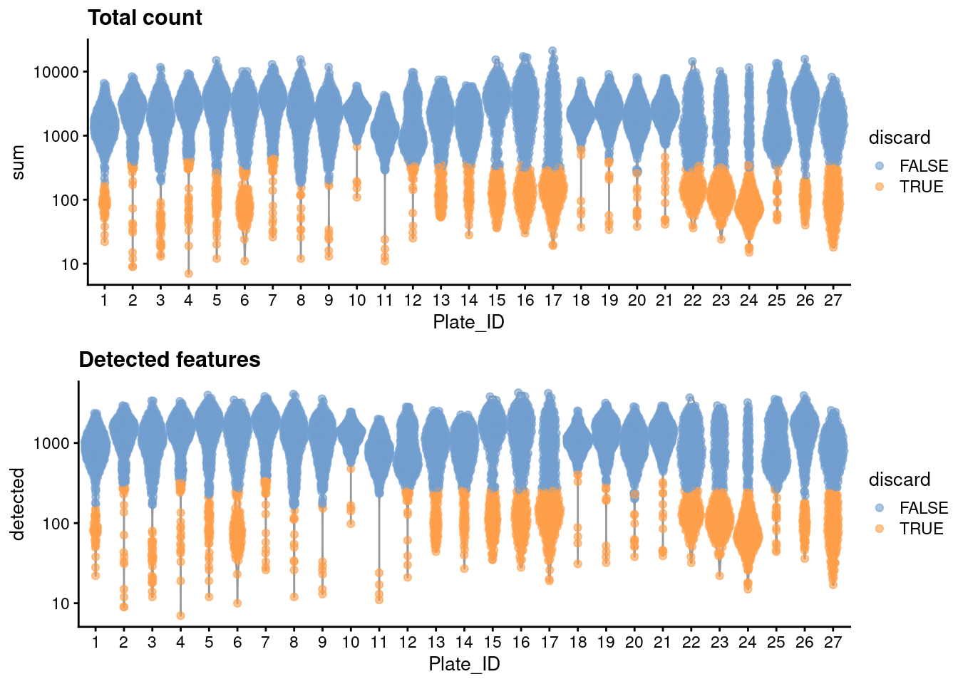
Figure 37.1: Distribution of each QC metric across cells in the Paul HSC dataset. Each point represents a cell and is colored according to whether that cell was discarded.
37.4 Normalization
library(scran)
set.seed(101000110)
clusters <- quickCluster(sce.paul)
sce.paul <- computeSumFactors(sce.paul, clusters=clusters)
sce.paul <- logNormCounts(sce.paul)
We examine some key metrics for the distribution of size factors, and compare it to the library sizes as a sanity check (Figure 37.2).
##    Min. 1st Qu.  Median    Mean 3rd Qu.    Max.
## 0.057 0.422 0.775 1.000 1.335 9.654plot(librarySizeFactors(sce.paul), sizeFactors(sce.paul), pch=16,
xlab="Library size factors", ylab="Deconvolution factors", log="xy")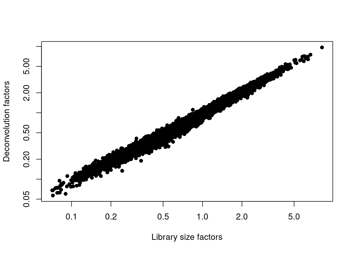
Figure 37.2: Relationship between the library size factors and the deconvolution size factors in the Paul HSC dataset.
37.5 Variance modelling
We fit a mean-variance trend to the endogenous genes to detect highly variable genes.
Unfortunately, the plates are confounded with an experimental treatment (Batch_desc) so we cannot block on the plate of origin.
set.seed(00010101)
dec.paul <- modelGeneVarByPoisson(sce.paul)
top.paul <- getTopHVGs(dec.paul, prop=0.1)plot(dec.paul$mean, dec.paul$total, pch=16, cex=0.5,
xlab="Mean of log-expression", ylab="Variance of log-expression")
curve(metadata(dec.paul)$trend(x), col="blue", add=TRUE)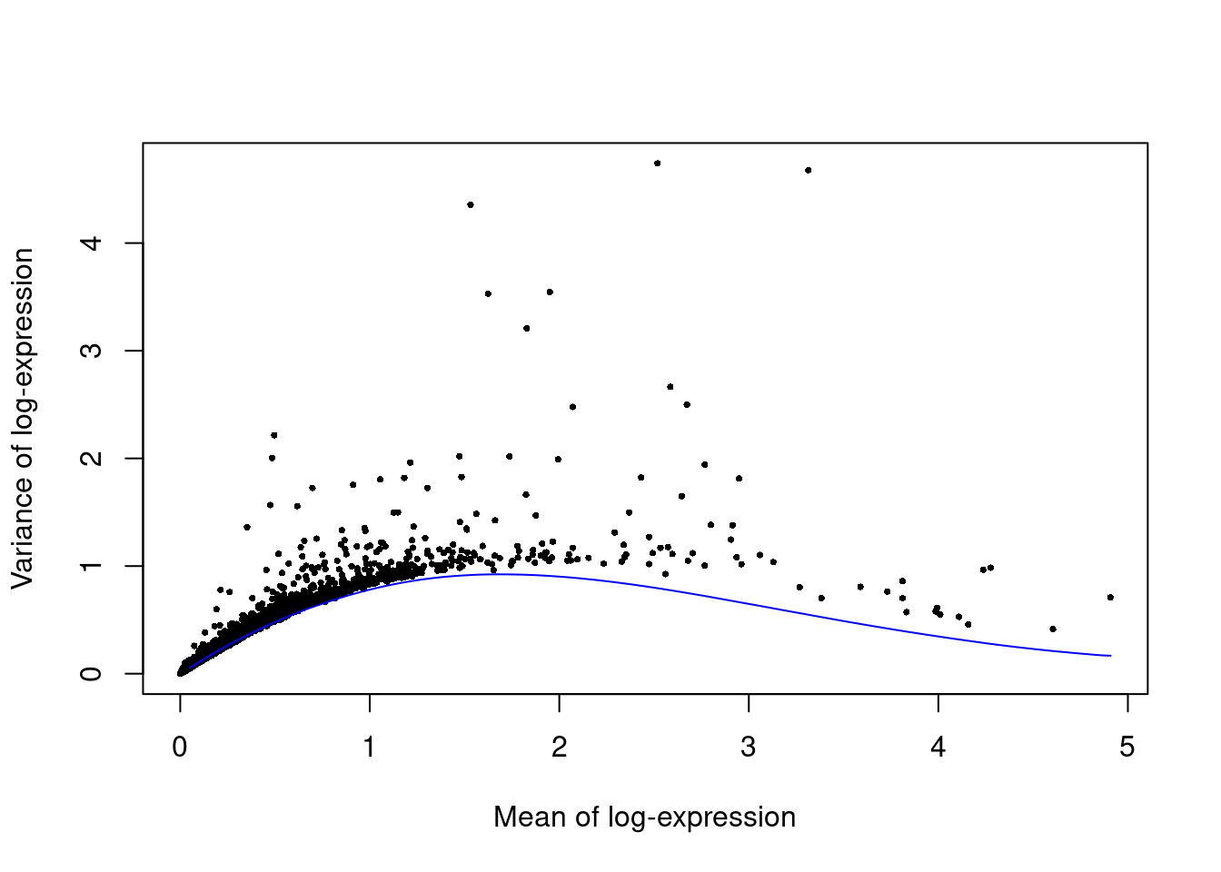
Figure 37.3: Per-gene variance as a function of the mean for the log-expression values in the Paul HSC dataset. Each point represents a gene (black) with the mean-variance trend (blue) fitted to simulated Poisson noise.
37.6 Dimensionality reduction
set.seed(101010011)
sce.paul <- denoisePCA(sce.paul, technical=dec.paul, subset.row=top.paul)
sce.paul <- runTSNE(sce.paul, dimred="PCA")
We check that the number of retained PCs is sensible.
## [1] 1337.7 Clustering
snn.gr <- buildSNNGraph(sce.paul, use.dimred="PCA", type="jaccard")
colLabels(sce.paul) <- factor(igraph::cluster_louvain(snn.gr)$membership)
These is a strong relationship between the cluster and the experimental treatment (Figure 37.4), which is to be expected. Of course, this may also be attributable to some batch effect; the confounded nature of the experimental design makes it difficult to make any confident statements either way.
tab <- table(colLabels(sce.paul), sce.paul$Batch_desc)
rownames(tab) <- paste("Cluster", rownames(tab))
pheatmap::pheatmap(log10(tab+10), color=viridis::viridis(100))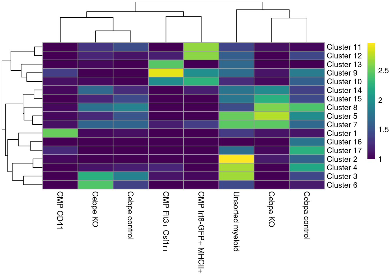
Figure 37.4: Heatmap of the distribution of cells across clusters (rows) for each experimental treatment (column).
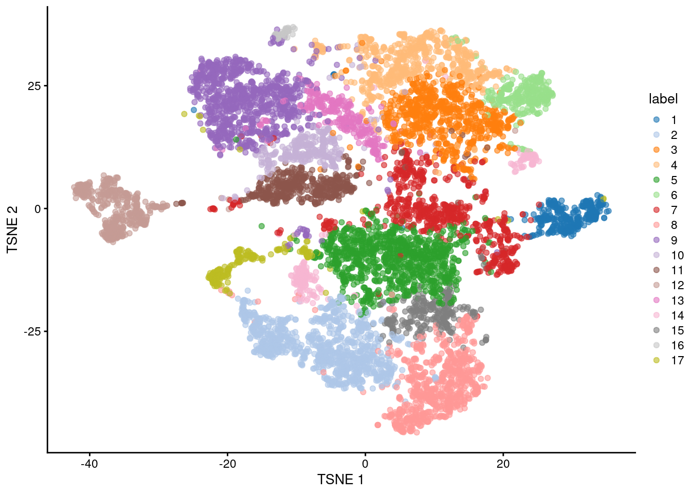
Figure 37.5: Obligatory \(t\)-SNE plot of the Paul HSC dataset, where each point represents a cell and is colored according to the assigned cluster.
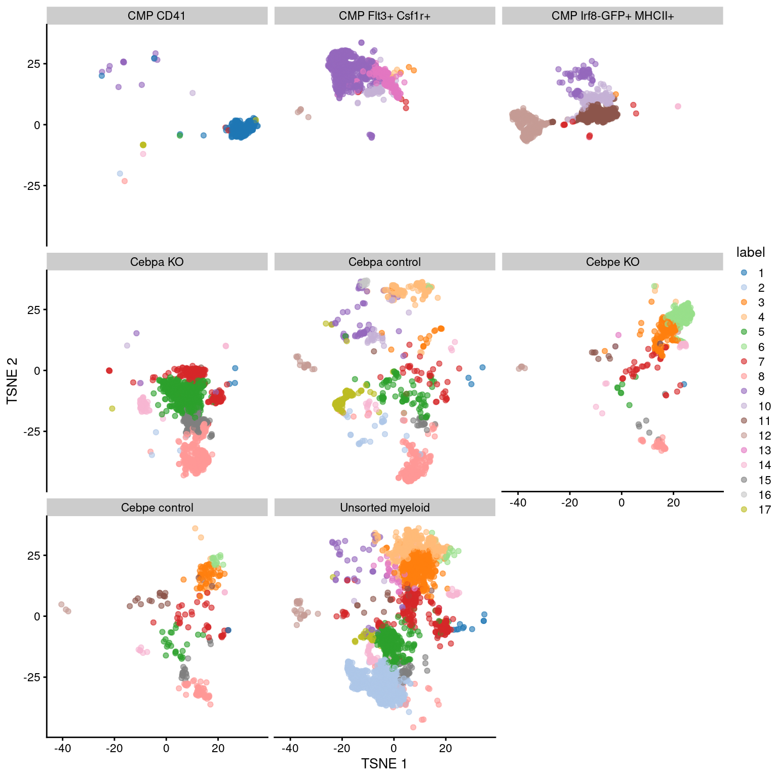
Figure 37.6: Obligatory \(t\)-SNE plot of the Paul HSC dataset faceted by the treatment condition, where each point represents a cell and is colored according to the assigned cluster.
Session Info
R version 4.0.4 (2021-02-15)
Platform: x86_64-pc-linux-gnu (64-bit)
Running under: Ubuntu 20.04.2 LTS

Matrix products: default
BLAS:   /home/biocbuild/bbs-3.12-books/R/lib/libRblas.so
LAPACK: /home/biocbuild/bbs-3.12-books/R/lib/libRlapack.so

locale:
 [1] LC_CTYPE=en_US.UTF-8       LC_NUMERIC=C
 [3] LC_TIME=en_US.UTF-8        LC_COLLATE=C
 [5] LC_MONETARY=en_US.UTF-8    LC_MESSAGES=en_US.UTF-8
 [7] LC_PAPER=en_US.UTF-8       LC_NAME=C
 [9] LC_ADDRESS=C               LC_TELEPHONE=C
[11] LC_MEASUREMENT=en_US.UTF-8 LC_IDENTIFICATION=C

attached base packages:
[1] parallel  stats4    stats     graphics  grDevices utils     datasets
[8] methods   base

other attached packages:
 [1] scran_1.18.5                scater_1.18.6
 [3] ggplot2_3.3.3               AnnotationHub_2.22.0
 [5] BiocFileCache_1.14.0        dbplyr_2.1.0
 [7] ensembldb_2.14.0            AnnotationFilter_1.14.0
 [9] GenomicFeatures_1.42.2      AnnotationDbi_1.52.0
[11] scRNAseq_2.4.0              SingleCellExperiment_1.12.0
[13] SummarizedExperiment_1.20.0 Biobase_2.50.0
[15] GenomicRanges_1.42.0        GenomeInfoDb_1.26.4
[17] IRanges_2.24.1              S4Vectors_0.28.1
[19] BiocGenerics_0.36.0         MatrixGenerics_1.2.1
[21] matrixStats_0.58.0          BiocStyle_2.18.1
[23] rebook_1.0.0

loaded via a namespace (and not attached):
  [1] igraph_1.2.6                  lazyeval_0.2.2
  [3] BiocParallel_1.24.1           digest_0.6.27
  [5] htmltools_0.5.1.1             viridis_0.5.1
  [7] fansi_0.4.2                   magrittr_2.0.1
  [9] memoise_2.0.0                 limma_3.46.0
 [11] Biostrings_2.58.0             askpass_1.1
 [13] prettyunits_1.1.1             colorspace_2.0-0
 [15] blob_1.2.1                    rappdirs_0.3.3
 [17] xfun_0.22                     dplyr_1.0.5
 [19] callr_3.5.1                   crayon_1.4.1
 [21] RCurl_1.98-1.3                jsonlite_1.7.2
 [23] graph_1.68.0                  glue_1.4.2
 [25] gtable_0.3.0                  zlibbioc_1.36.0
 [27] XVector_0.30.0                DelayedArray_0.16.2
 [29] BiocSingular_1.6.0            scales_1.1.1
 [31] pheatmap_1.0.12               edgeR_3.32.1
 [33] DBI_1.1.1                     Rcpp_1.0.6
 [35] viridisLite_0.3.0             xtable_1.8-4
 [37] progress_1.2.2                dqrng_0.2.1
 [39] bit_4.0.4                     rsvd_1.0.3
 [41] httr_1.4.2                    RColorBrewer_1.1-2
 [43] ellipsis_0.3.1                pkgconfig_2.0.3
 [45] XML_3.99-0.6                  farver_2.1.0
 [47] scuttle_1.0.4                 CodeDepends_0.6.5
 [49] sass_0.3.1                    locfit_1.5-9.4
 [51] utf8_1.2.1                    labeling_0.4.2
 [53] tidyselect_1.1.0              rlang_0.4.10
 [55] later_1.1.0.1                 munsell_0.5.0
 [57] BiocVersion_3.12.0            tools_4.0.4
 [59] cachem_1.0.4                  generics_0.1.0
 [61] RSQLite_2.2.4                 ExperimentHub_1.16.0
 [63] evaluate_0.14                 stringr_1.4.0
 [65] fastmap_1.1.0                 yaml_2.2.1
 [67] processx_3.4.5                knitr_1.31
 [69] bit64_4.0.5                   purrr_0.3.4
 [71] sparseMatrixStats_1.2.1       mime_0.10
 [73] xml2_1.3.2                    biomaRt_2.46.3
 [75] compiler_4.0.4                beeswarm_0.3.1
 [77] curl_4.3                      interactiveDisplayBase_1.28.0
 [79] statmod_1.4.35                tibble_3.1.0
 [81] bslib_0.2.4                   stringi_1.5.3
 [83] highr_0.8                     ps_1.6.0
 [85] lattice_0.20-41               bluster_1.0.0
 [87] ProtGenerics_1.22.0           Matrix_1.3-2
 [89] vctrs_0.3.6                   pillar_1.5.1
 [91] lifecycle_1.0.0               BiocManager_1.30.10
 [93] jquerylib_0.1.3               BiocNeighbors_1.8.2
 [95] cowplot_1.1.1                 bitops_1.0-6
 [97] irlba_2.3.3                   httpuv_1.5.5
 [99] rtracklayer_1.50.0            R6_2.5.0
[101] bookdown_0.21                 promises_1.2.0.1
[103] gridExtra_2.3                 vipor_0.4.5
[105] codetools_0.2-18              assertthat_0.2.1
[107] openssl_1.4.3                 withr_2.4.1
[109] GenomicAlignments_1.26.0      Rsamtools_2.6.0
[111] GenomeInfoDbData_1.2.4        hms_1.0.0
[113] grid_4.0.4                    beachmat_2.6.4
[115] rmarkdown_2.7                 DelayedMatrixStats_1.12.3
[117] Rtsne_0.15                    shiny_1.6.0
[119] ggbeeswarm_0.6.0
Bibliography
Paul, F., Y. Arkin, A. Giladi, D. A. Jaitin, E. Kenigsberg, H. Keren-Shaul, D. Winter, et al. 2015. “Transcriptional Heterogeneity and Lineage Commitment in Myeloid Progenitors.” Cell 163 (7): 1663–77.