Chapter 15 Droplet processing
15.1 Motivation
Droplet-based single-cell protocols aim to isolate each cell inside its own droplet in a water-in-oil emulsion, such that each droplet serves as a miniature reaction chamber for highly multiplexed library preparation (Macosko et al. 2015; Klein et al. 2015). Upon sequencing, reads are assigned to individual cells based on the presence of droplet-specific barcodes. This enables a massive increase in the number of cells that can be processed in typical scRNA-seq experiments, contributing to the dominance3 of technologies such as the 10X Genomics platform (Zheng et al. 2017). However, as the allocation of cells to droplets is not known in advance, the data analysis requires some special steps to determine what each droplet actually contains. This chapter explores some of the more common preprocessing procedures that might be applied to the count matrices generated from droplet protocols.
15.2 Calling cells from empty droplets
15.2.1 Background
An unique aspect of droplet-based data is that we have no prior knowledge about whether a particular library (i.e., cell barcode) corresponds to cell-containing or empty droplets. Thus, we need to call cells from empty droplets based on the observed expression profiles. This is not entirely straightforward as empty droplets can contain ambient (i.e., extracellular) RNA that can be captured and sequenced, resulting in non-zero counts for libraries that do not contain any cell. To demonstrate, we obtain the unfiltered count matrix for the PBMC dataset from 10X Genomics.
#--- loading ---#
library(DropletTestFiles)
raw.path <- getTestFile("tenx-2.1.0-pbmc4k/1.0.0/raw.tar.gz")
out.path <- file.path(tempdir(), "pbmc4k")
untar(raw.path, exdir=out.path)

library(DropletUtils)
fname <- file.path(out.path, "raw_gene_bc_matrices/GRCh38")
sce.pbmc <- read10xCounts(fname, col.names=TRUE)## class: SingleCellExperiment
## dim: 33694 737280
## metadata(1): Samples
## assays(1): counts
## rownames(33694): ENSG00000243485 ENSG00000237613 ... ENSG00000277475
## ENSG00000268674
## rowData names(2): ID Symbol
## colnames(737280): AAACCTGAGAAACCAT-1 AAACCTGAGAAACCGC-1 ...
## TTTGTCATCTTTAGTC-1 TTTGTCATCTTTCCTC-1
## colData names(2): Sample Barcode
## reducedDimNames(0):
## altExpNames(0):The distribution of total counts exhibits a sharp transition between barcodes with large and small total counts (Figure 15.1), probably corresponding to cell-containing and empty droplets respectively. A simple approach would be to apply a threshold on the total count to only retain those barcodes with large totals. However, this unnecessarily discards libraries derived from cell types with low RNA content.
library(DropletUtils)
bcrank <- barcodeRanks(counts(sce.pbmc))

# Only showing unique points for plotting speed.
uniq <- !duplicated(bcrank$rank)
plot(bcrank$rank[uniq], bcrank$total[uniq], log="xy",
    xlab="Rank", ylab="Total UMI count", cex.lab=1.2)

abline(h=metadata(bcrank)$inflection, col="darkgreen", lty=2)
abline(h=metadata(bcrank)$knee, col="dodgerblue", lty=2)

legend("bottomleft", legend=c("Inflection", "Knee"),
        col=c("darkgreen", "dodgerblue"), lty=2, cex=1.2)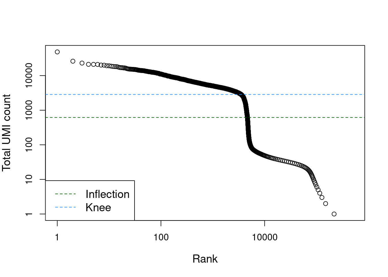
Figure 15.1: Total UMI count for each barcode in the PBMC dataset, plotted against its rank (in decreasing order of total counts). The inferred locations of the inflection and knee points are also shown.
15.2.2 Testing for empty droplets
We use the emptyDrops() function to test whether the expression profile for each cell barcode is significantly different from the ambient RNA pool (Lun et al. 2019).
Any significant deviation indicates that the barcode corresponds to a cell-containing droplet.
This allows us to discriminate between well-sequenced empty droplets and droplets derived from cells with little RNA, both of which would have similar total counts in Figure 15.1.
We call cells at a false discovery rate (FDR) of 0.1%, meaning that no more than 0.1% of our called barcodes should be empty droplets on average.
# emptyDrops performs Monte Carlo simulations to compute p-values,
# so we need to set the seed to obtain reproducible results.
set.seed(100)
e.out <- emptyDrops(counts(sce.pbmc))

# See ?emptyDrops for an explanation of why there are NA values.
summary(e.out$FDR <= 0.001)
## Mode FALSE TRUE NA's
## logical 989 4300 731991emptyDrops() uses Monte Carlo simulations to compute \(p\)-values for the multinomial sampling transcripts from the ambient pool.
The number of Monte Carlo iterations determines the lower bound for the \(p\)-values (Phipson and Smyth 2010).
The Limited field in the output indicates whether or not the computed \(p\)-value for a particular barcode is bounded by the number of iterations.
If any non-significant barcodes are TRUE for Limited, we may need to increase the number of iterations.
A larger number of iterations will result in a lower \(p\)-value for these barcodes, which may allow them to be detected after correcting for multiple testing.
##        Limited
## Sig     FALSE TRUE
##   FALSE   989    0
##   TRUE   1728 2572
As mentioned above, emptyDrops() assumes that barcodes with low total UMI counts are empty droplets.
Thus, the null hypothesis should be true for all of these barcodes.
We can check whether the hypothesis testing procedure holds its size by examining the distribution of \(p\)-values for low-total barcodes with test.ambient=TRUE.
Ideally, the distribution should be close to uniform (Figure 15.2).
Large peaks near zero indicate that barcodes with total counts below lower are not all ambient in origin.
This can be resolved by decreasing lower further to ensure that barcodes corresponding to droplets with very small cells are not used to estimate the ambient profile.
set.seed(100)
limit <- 100
all.out <- emptyDrops(counts(sce.pbmc), lower=limit, test.ambient=TRUE)
hist(all.out$PValue[all.out$Total <= limit & all.out$Total > 0],
xlab="P-value", main="", col="grey80") 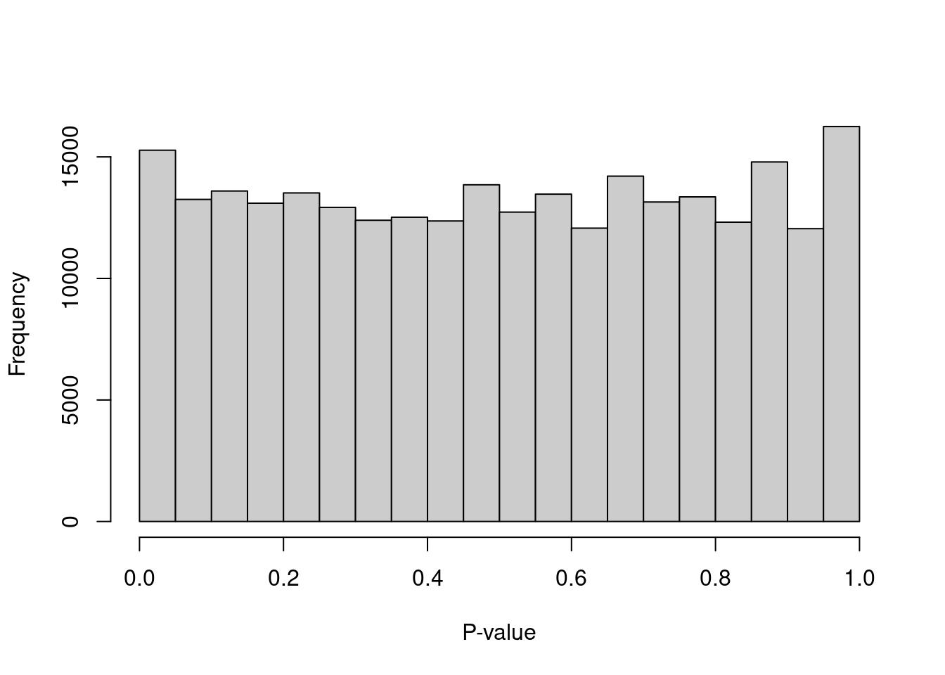
Figure 15.2: Distribution of \(p\)-values for the assumed empty droplets.
Once we are satisfied with the performance of emptyDrops(), we subset our SingleCellExperiment object to retain only the detected cells.
Discerning readers will notice the use of which(), which conveniently removes the NAs prior to the subsetting.
It usually only makes sense to call cells using a count matrix involving libraries from a single sample. The composition of transcripts in the ambient solution will usually between samples, so the same ambient profile cannot be reused. If multiple samples are present in a dataset, their counts should only be combined after cell calling is performed on each matrix.
15.2.3 Relationship with other QC metrics
While emptyDrops() will distinguish cells from empty droplets, it makes no statement about the quality of the cells.
It is entirely possible for droplets to contain damaged or dying cells, which need to be removed prior to downstream analysis.
This is achieved using the same outlier-based strategy described in Section 6.3.2.
Filtering on the mitochondrial proportion provides the most additional benefit in this situation, provided that we check that we are not removing a subpopulation of metabolically active cells (Figure 15.3).
library(scuttle)
is.mito <- grep("^MT-", rowData(sce.pbmc)$Symbol)
pbmc.qc <- perCellQCMetrics(sce.pbmc, subsets=list(MT=is.mito))
discard.mito <- isOutlier(pbmc.qc$subsets_MT_percent, type="higher")
summary(discard.mito)
## Mode FALSE TRUE
## logical 3985 315plot(pbmc.qc$sum, pbmc.qc$subsets_MT_percent, log="x",
xlab="Total count", ylab='Mitochondrial %')
abline(h=attr(discard.mito, "thresholds")["higher"], col="red")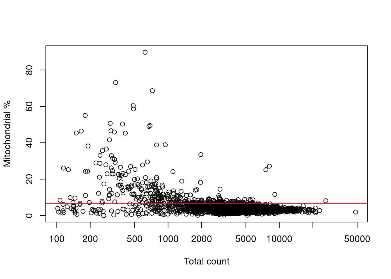
Figure 15.3: Percentage of reads assigned to mitochondrial transcripts, plotted against the library size. The red line represents the upper threshold used for QC filtering.
emptyDrops() already removes cells with very low library sizes or (by association) low numbers of expressed genes.
Thus, further filtering on these metrics is not strictly necessary.
It may still be desirable to filter on both of these metrics to remove non-empty droplets containing cell fragments or stripped nuclei that were not caught by the mitochondrial filter.
However, this should be weighed against the risk of losing genuine cell types as discussed in Section 6.3.2.2.
Note that CellRanger version 3 automatically performs cell calling using an algorithm similar to emptyDrops().
If we had started our analysis with the filtered count matrix, we could go straight to computing other QC metrics.
We would not need to run emptyDrops() manually as shown here, and indeed, attempting to do so would lead to nonsensical results if not outright software errors.
Nonetheless, it may still be desirable to load the unfiltered matrix and apply emptyDrops() ourselves, on occasions where more detailed inspection or control of the cell-calling statistics is desired.
15.3 Removing ambient contamination
For routine analyses, there is usually no need to remove the ambient contamination from each library. A consistent level of contamination across the dataset does not introduce much spurious heterogeneity, so dimensionality reduction and clustering on the original (log-)expression matrix remain valid. For genes that are highly abundant in the ambient solution, we can expect some loss of signal due to shrinkage of the log-fold changes between clusters towards zero, but this effect should be negligible for any genes that are so strongly upregulated that they are able to contribute to the ambient solution in the first place. This suggests that ambient removal can generally be omitted from most analyses, though we will describe it here regardless as it can be useful in specific situations.
Effective removal of ambient contamination involves tackling a number of issues. We need to know how much contamination is present in each cell, which usually requires some prior biological knowledge about genes that should not be expressed in the dataset (e.g., mitochondrial genes in single-nuclei datasets, see Section 19.4) or genes with mutually exclusive expression profiles (Young and Behjati 2018). Those same genes must be highly abundant in the ambient solution to have enough counts in each cell for precise estimation of the scale of the contamination. The actual subtraction of the ambient contribution also must be done in a manner that respects the mean-variance relationship of the count data. Unfortunately, these issues are difficult to address for single-cell data due to the imprecision of low counts,
Rather than attempting to remove contamination from individual cells, a more measured approach is to operate on clusters of related cells.
The removeAmbience() function from DropletUtils will remove the contamination from the cluster-level profiles and propagate the effect of those changes back to the individual cells.
Specifically, given a count matrix for a single sample and its associated ambient profile, removeAmbience() will:
- Aggregate counts in each cluster to obtain an average profile per cluster.
- Estimate the contamination proportion in each cluster with
maximumAmbience()(see Section 14.4). This has the useful property of not requiring any prior knowledge of control or mutually exclusive expression profiles, albeit at the cost of some statistical rigor. - Subtract the estimated contamination from the cluster-level average.
- Perform quantile-quantile mapping of each individual cell’s counts from the old average to the new subtracted average. This preserves the mean-variance relationship while yielding corrected single-cell profiles.
We demonstrate this process on our PBMC dataset below.
#--- loading ---#
library(DropletTestFiles)
raw.path <- getTestFile("tenx-2.1.0-pbmc4k/1.0.0/raw.tar.gz")
out.path <- file.path(tempdir(), "pbmc4k")
untar(raw.path, exdir=out.path)

library(DropletUtils)
fname <- file.path(out.path, "raw_gene_bc_matrices/GRCh38")
sce.pbmc <- read10xCounts(fname, col.names=TRUE)

#--- gene-annotation ---#
library(scater)
rownames(sce.pbmc) <- uniquifyFeatureNames(
    rowData(sce.pbmc)$ID, rowData(sce.pbmc)$Symbol)

library(EnsDb.Hsapiens.v86)
location <- mapIds(EnsDb.Hsapiens.v86, keys=rowData(sce.pbmc)$ID,
    column="SEQNAME", keytype="GENEID")

#--- cell-detection ---#
set.seed(100)
e.out <- emptyDrops(counts(sce.pbmc))
sce.pbmc <- sce.pbmc[,which(e.out$FDR <= 0.001)]

#--- quality-control ---#
stats <- perCellQCMetrics(sce.pbmc, subsets=list(Mito=which(location=="MT")))
high.mito <- isOutlier(stats$subsets_Mito_percent, type="higher")
sce.pbmc <- sce.pbmc[,!high.mito]

#--- normalization ---#
library(scran)
set.seed(1000)
clusters <- quickCluster(sce.pbmc)
sce.pbmc <- computeSumFactors(sce.pbmc, cluster=clusters)
sce.pbmc <- logNormCounts(sce.pbmc)

#--- variance-modelling ---#
set.seed(1001)
dec.pbmc <- modelGeneVarByPoisson(sce.pbmc)
top.pbmc <- getTopHVGs(dec.pbmc, prop=0.1)

#--- dimensionality-reduction ---#
set.seed(10000)
sce.pbmc <- denoisePCA(sce.pbmc, subset.row=top.pbmc, technical=dec.pbmc)

set.seed(100000)
sce.pbmc <- runTSNE(sce.pbmc, dimred="PCA")

set.seed(1000000)
sce.pbmc <- runUMAP(sce.pbmc, dimred="PCA")

#--- clustering ---#
g <- buildSNNGraph(sce.pbmc, k=10, use.dimred = 'PCA')
clust <- igraph::cluster_walktrap(g)$membership
colLabels(sce.pbmc) <- factor(clust)
# Not all genes are reported in the ambient profile from emptyDrops,
# as genes with counts of zero across all droplets are just removed.
# So for convenience, we will restrict our analysis to genes with
# non-zero counts in at least one droplet (empty or otherwise).
amb <- metadata(e.out)$ambient[,1]
stripped <- sce.pbmc[names(amb),]
out <- removeAmbience(counts(stripped), ambient=amb, groups=colLabels(stripped))
dim(out)## [1] 20112 3985We can visualize the effects of ambient removal on a gene like IGKC, which presumably should only be expressed in the B cell lineage. This gene has some level of expression in each cluster in the original dataset but is “zeroed” in most clusters after removal (Figure 15.4).
library(scater)
counts(stripped, withDimnames=FALSE) <- out
stripped <- logNormCounts(stripped)

gridExtra::grid.arrange(
    plotExpression(sce.pbmc, x="label", colour_by="label", features="IGKC") +
        ggtitle("Before"),
    plotExpression(stripped, x="label", colour_by="label", features="IGKC") +
        ggtitle("After"),
    ncol=2
)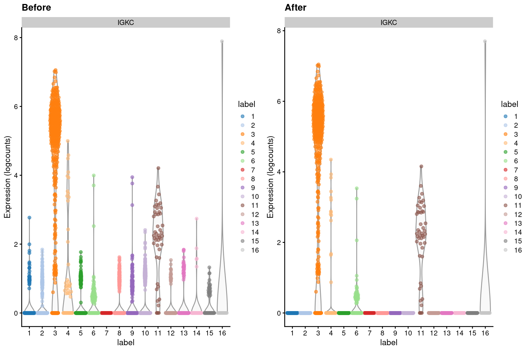
Figure 15.4: Distribution of IGKC log-expression values in each cluster of the PBMC dataset, before and after removal of ambient contamination.
We observe a similar phenomenon with the LYZ gene (Figure 15.5), which should only be expressed in macrophages and neutrophils.
In fact, if we knew this beforehand, we could specify these two mutually exclusive sets - i.e., LYZ and IGKC and their related genes - in the features= argument to removeAmbience().
This knowledge is subsequently used to estimate the contamination in each cluster, an approach that is more conceptually similar to the methods in the SoupX package.
gridExtra::grid.arrange(
    plotExpression(sce.pbmc, x="label", colour_by="label", features="LYZ") +
        ggtitle("Before"),
    plotExpression(stripped, x="label", colour_by="label", features="LYZ") +
        ggtitle("After"),
    ncol=2
)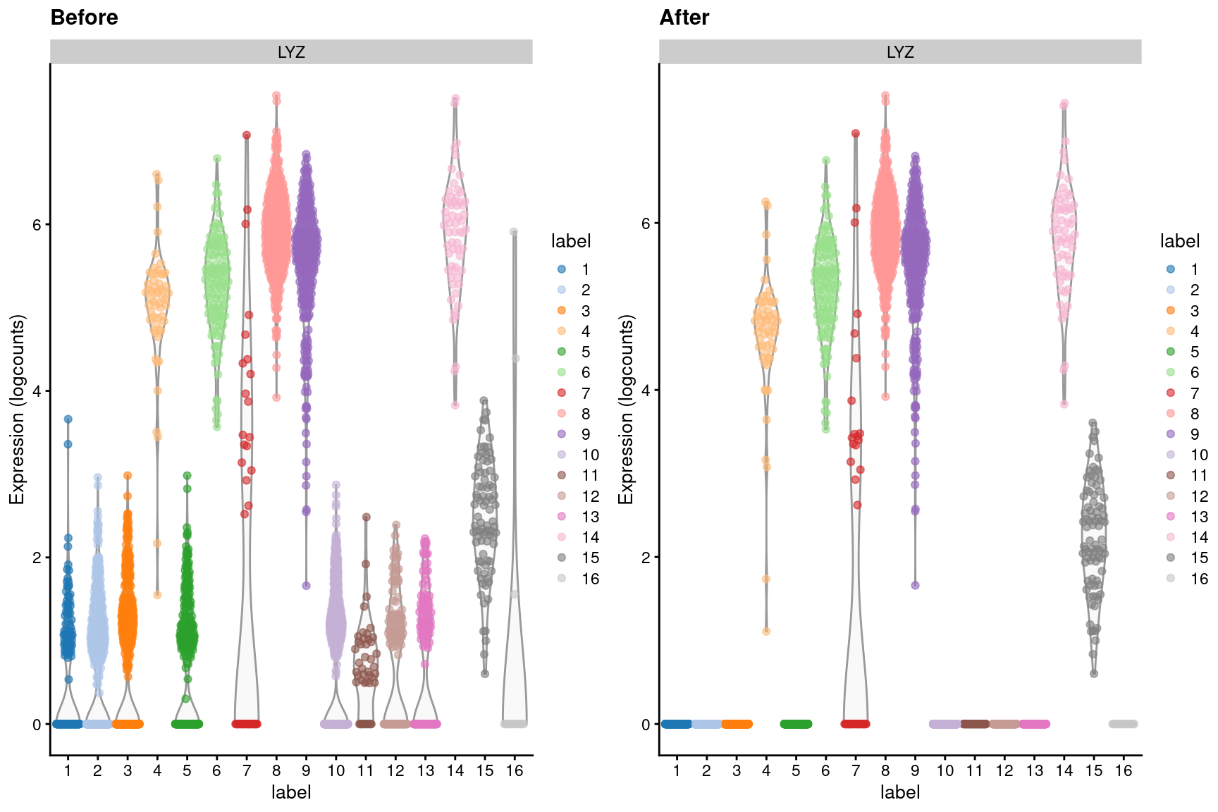
Figure 15.5: Distribution of LYZ log-expression values in each cluster of the PBMC dataset, before and after removal of ambient contamination.
While these results look impressive, discerning readers will note that the method relies on having sensible clusters.
This limits the function’s applicability to the end of an analysis after all the characterization has already been done.
As such, the stripped matrix can really only be used in downstream steps like the DE analysis (where it is unlikely to have much effect beyond inflating already-large log-fold changes) or - most importantly - in visualization, where users can improve the aesthetics of their plots by eliminating harmless background expression.
Of course, one could repeat the entire analysis on the stripped count matrix to obtain new clusters, but this seems unnecessarily circuituous, especially if the clusters were deemed good enough for use in removeAmbience() in the first place.
Finally, it may be worth considering whether a corrected per-cell count matrix is really necessary.
In removeAmbience(), counts for each gene are assumed to follow a negative binomial distribution with a fixed dispersion.
This is necessary to perform the quantile-quantile remapping to obtain a corrected version of each individual cell’s counts, but violations of these distributional assumptions will introduce inaccuracies in downstream models.
Some analyses may have specific remedies to ambient contamination that do not require corrected per-cell counts (Section 14.4), so we can avoid these assumptions altogether if such remedies are available.
15.4 Demultiplexing cell hashes
15.4.1 Background
Cell hashing (Stoeckius et al. 2018) is a useful technique that allows cells from different samples to be processed in a single run of a droplet-based protocol. Cells from a single sample are first labelled with a unique hashing tag oligo (HTOs), usually via conjugation of the HTO to an antibody against a ubiquitous surface marker or a membrane-binding compound like cholesterol (McGinnis et al. 2019). Cells from different samples are then mixed together and the multiplexed pool is used for droplet-based library preparation; each cell is assigned back to its sample of origin based on its most abundant HTO. By processing multiple samples together, we can avoid batch effects and simplify the logistics of studies with a large number of samples.
Sequencing of the HTO-derived cDNA library yields a count matrix where each row corresponds to a HTO and each column corresponds to a cell barcode.
This can be stored as an alternative Experiment in our SingleCellExperiment, alongside the main experiment containing the counts for the actual genes.
We demonstrate on some data from the original Stoeckius et al. (2018) study, which contains counts for a mixture of 4 cell lines across 12 samples.
## class: SingleCellExperiment
## dim: 25339 25088
## metadata(0):
## assays(1): counts
## rownames(25339): A1BG A1BG-AS1 ... snoU2-30 snoZ178
## rowData names(0):
## colnames(25088): CAGATCAAGTAGGCCA CCTTTCTGTCGGATCC ... CGGTTATCCATCTGCT
##   CGGTTCACACGTCAGC
## colData names(0):
## reducedDimNames(0):
## altExpNames(1): hto## class: SingleCellExperiment
## dim: 12 25088
## metadata(0):
## assays(1): counts
## rownames(12): HEK_A HEK_B ... KG1_B KG1_C
## rowData names(0):
## colnames(25088): CAGATCAAGTAGGCCA CCTTTCTGTCGGATCC ... CGGTTATCCATCTGCT
## CGGTTCACACGTCAGC
## colData names(0):
## reducedDimNames(0):
## altExpNames(0):## CAGATCAAGTAGGCCA CCTTTCTGTCGGATCC CATATGGCATGGAATA
## HEK_A 1 0 0
## HEK_B 111 0 1
## HEK_C 7 1 7
## THP1_A 15 19 16
## THP1_B 10 8 5
## THP1_C 4 3 6
## K562_A 118 0 245
## K562_B 5 530 131
## K562_C 1 3 4
## KG1_A 30 25 24
## KG1_B 40 14 239
## KG1_C 32 36 3815.4.2 Cell calling options
Our first task is to identify the libraries corresponding to cell-containing droplets.
This can be applied on the gene count matrix or the HTO count matrix, depending on what information we have available.
We start with the usual application of emptyDrops() on the gene count matrix of hto.sce (Figure 15.6).
set.seed(10010)
e.out.gene <- emptyDrops(counts(hto.sce))
is.cell <- e.out.gene$FDR <= 0.001
summary(is.cell)
## Mode FALSE TRUE NA's
## logical 1384 7934 15770par(mfrow=c(1,2))
r <- rank(-e.out.gene$Total)
plot(r, e.out.gene$Total, log="xy", xlab="Rank", ylab="Total gene count", main="")
abline(h=metadata(e.out.gene)$retain, col="darkgrey", lty=2, lwd=2)
hist(log10(e.out.gene$Total[is.cell]), xlab="Log[10] gene count", main="")
Figure 15.6: Cell-calling statistics from running emptyDrops() on the gene count in the cell line mixture data. Left: Barcode rank plot with the estimated knee point in grey. Right: distribution of log-total counts for libraries identified as cells.
Alternatively, we could also apply emptyDrops() to the HTO count matrix but this is slightly more complicated.
As HTOs are sequenced separately from the endogenous transcripts, the coverage of the former is less predictable across studies; this makes it difficult to determine an appropriate default value of lower= for estimation of the initial ambient profile.
We instead estimate the ambient profile by excluding the top by.rank= barcodes with the largest totals, under the assumption that no more than by.rank= cells were loaded.
Here we have chosen 12000, which is largely a guess to ensure that we can directly pick the knee point (Figure 15.7) in this somewhat pre-filtered dataset.
set.seed(10010)

# Setting lower= for correct knee point detection,
# as the coverage in this dataset is particularly low.
e.out.hto <- emptyDrops(counts(altExp(hto.sce)), by.rank=12000, lower=10)
summary(is.cell.hto <- e.out.hto$FDR <= 0.001)
## Mode FALSE TRUE NA's
## logical 2967 8955 13166par(mfrow=c(1,2))
r <- rank(-e.out.hto$Total)
plot(r, e.out.hto$Total, log="xy", xlab="Rank", ylab="Total HTO count", main="")
abline(h=metadata(e.out.hto)$retain, col="darkgrey", lty=2, lwd=2)
hist(log10(e.out.hto$Total[is.cell.hto]), xlab="Log[10] HTO count", main="")
Figure 15.7: Cell-calling statistics from running emptyDrops() on the HTO counts in the cell line mixture data. Left: Barcode rank plot with the knee point shown in grey. Right: distribution of log-total counts for libraries identified as cells.
While both approaches are valid, we tend to favor the cell calls derived from the gene matrix as this directly indicates that a cell is present in the droplet.
Indeed, at least a few libraries have very high total HTO counts yet very low total gene counts (Figure 15.8), suggesting that the presence of HTOs may not always equate to successful capture of that cell’s transcriptome.
HTO counts also tend to exhibit stronger overdispersion (i.e., lower alpha in the emptyDrops() calculations), increasing the risk of violating emptyDrops()’s distributional assumptions.
##        Genes
## HTO     FALSE  TRUE  <NA>
##   FALSE   342   798  1827
##   TRUE    200  6777  1978
## <NA> 842 359 11965plot(e.out.gene$Total, e.out.hto$Total, log="xy",
xlab="Total gene count", ylab="Total HTO count")
abline(v=metadata(e.out.gene)$lower, col="red", lwd=2, lty=2)
abline(h=metadata(e.out.hto)$lower, col="blue", lwd=2, lty=2)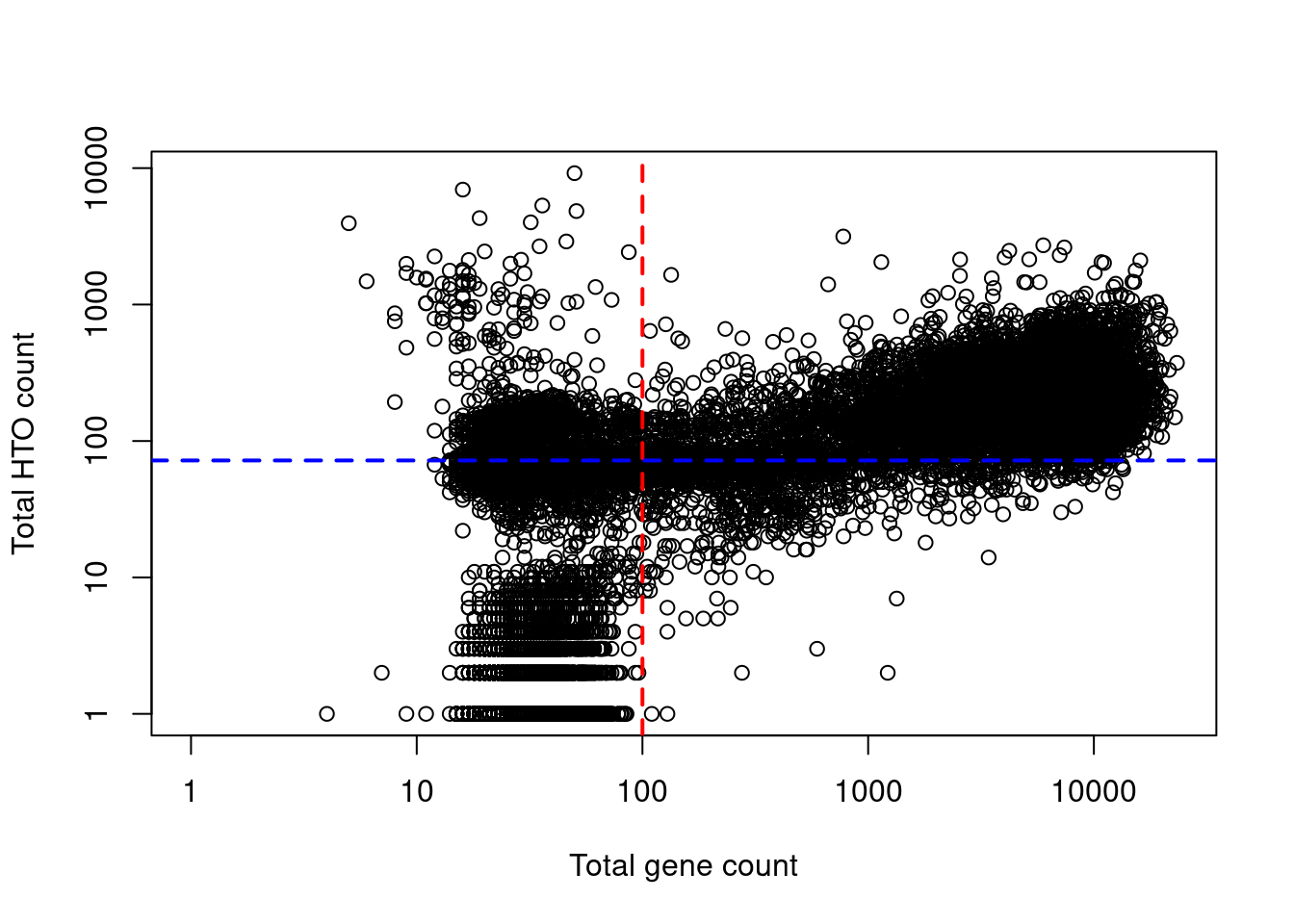
Figure 15.8: Total HTO counts plotted against the total gene counts for each library in the cell line mixture dataset. Each point represents a library while the dotted lines represent the thresholds below which libraries were assumed to be empty droplets.
Again, note that if we are picking up our analysis after processing with pipelines like CellRanger, it may be that the count matrix has already been subsetted to the cell-containing libraries. If so, we can skip this section entirely and proceed straight to demultiplexing.
15.4.3 Demultiplexing on HTO abundance
We run hashedDrops() to demultiplex the HTO count matrix for the subset of cell-containing libraries.
This reports the likely sample of origin for each library based on its most abundant HTO after adjusting those abundances for ambient contamination.
For quality control, it returns the log-fold change between the first and second-most abundant HTOs in each barcode libary (Figure 15.9), allowing us to quantify the certainty of each assignment.
hto.mat <- counts(altExp(hto.sce))[,which(is.cell)]
hash.stats <- hashedDrops(hto.mat)
hist(hash.stats$LogFC, xlab="Log fold-change from best to second HTO", main="")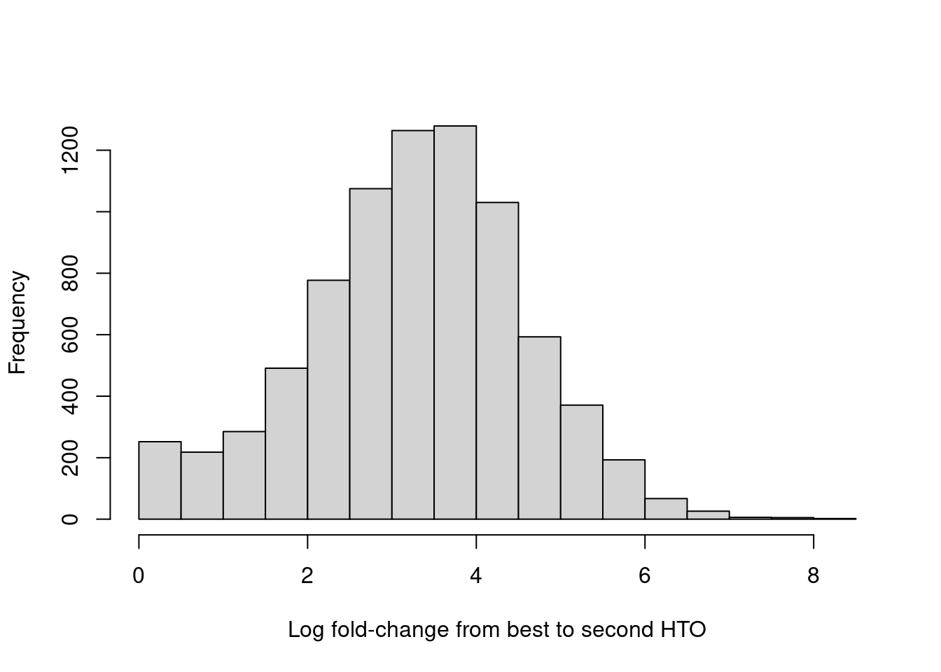
Figure 15.9: Distribution of log-fold changes from the first to second-most abundant HTO in each cell.
Confidently assigned cells should have large log-fold changes between the best and second-best HTO abundances as there should be exactly one dominant HTO per cell.
These are marked as such by the Confident field in the output of hashedDrops(), which can be used to filter out ambiguous assignments prior to downstream analyses.
##
##   1   2   3   4   5   6   7   8   9  10  11  12
## 664 732 636 595 629 655 570 684 603 726 662 778
# Confident assignments based on (i) a large log-fold change
# and (ii) not being a doublet.
table(hash.stats$Best[hash.stats$Confident])##
## 1 2 3 4 5 6 7 8 9 10 11 12
## 580 619 560 524 553 573 379 605 427 640 556 607In the absence of an a priori ambient profile, hashedDrops() will attempt to automatically estimate it from the count matrix.
This is done by assuming that each HTO has a bimodal distribution where the lower peak corresponds to ambient contamination in cells that do not belong to that HTO’s sample.
Counts are then averaged across all cells in the lower mode to obtain the relative abundance of that HTO (Figure 15.10).
hashedDrops() uses the ambient profile to adjust for systematic differences in HTO concentrations that could otherwise skew the log-fold changes -
for example, this particular dataset exhibits order-of-magnitude differences in the concentration of different HTOs.
The adjustment process itself involves a fair number of assumptions that we will not discuss here; see ?hashedDrops for more details.
barplot(metadata(hash.stats)$ambient, las=2,
    ylab="Inferred proportion of counts in the ambient solution")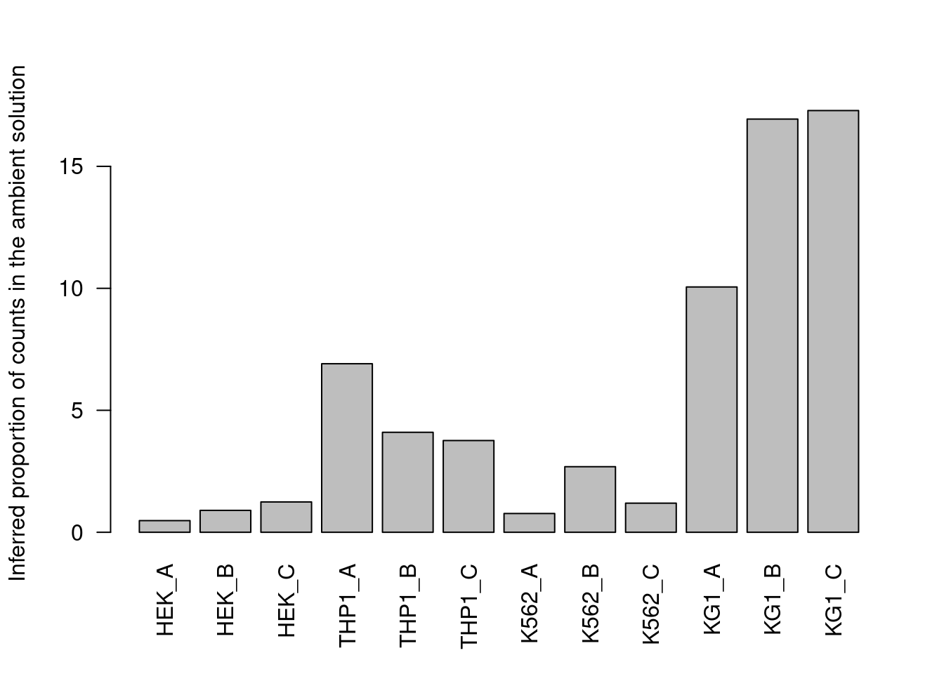
Figure 15.10: Proportion of each HTO in the ambient solution for the cell line mixture data, estimated from the HTO counts of cell-containing droplets.
If we are dealing with unfiltered data, we have the opportunity to improve the inferences by defining the ambient profile beforehand based on the empty droplets.
This simply involves summing the counts for each HTO across all known empty droplets, marked as those libraries with NA FDR values in the emptyDrops() output.
Alternatively, if we had called emptyDrops() directly on the HTO count matrix, we could just extract the ambient profile from the output’s metadata().
For this dataset, all methods agree well (Figure 15.10) though providing an a priori profile can be helpful in more extreme situations where the automatic method fails,
e.g., if there are too few cells in the lower mode for accurate estimation of a HTO’s ambient concentration.
estimates <- rbind(
    `Bimodal`=proportions(metadata(hash.stats)$ambient),
    `Empty (genes)`=proportions(rowSums(counts(altExp(hto.sce))[,is.na(e.out.gene$FDR)])),
    `Empty (HTO)`=metadata(e.out.hto)$ambient[,1]
)

barplot(estimates, beside=TRUE, ylab="Proportion of counts in the ambient solution")
legend("topleft", fill=gray.colors(3), legend=rownames(estimates))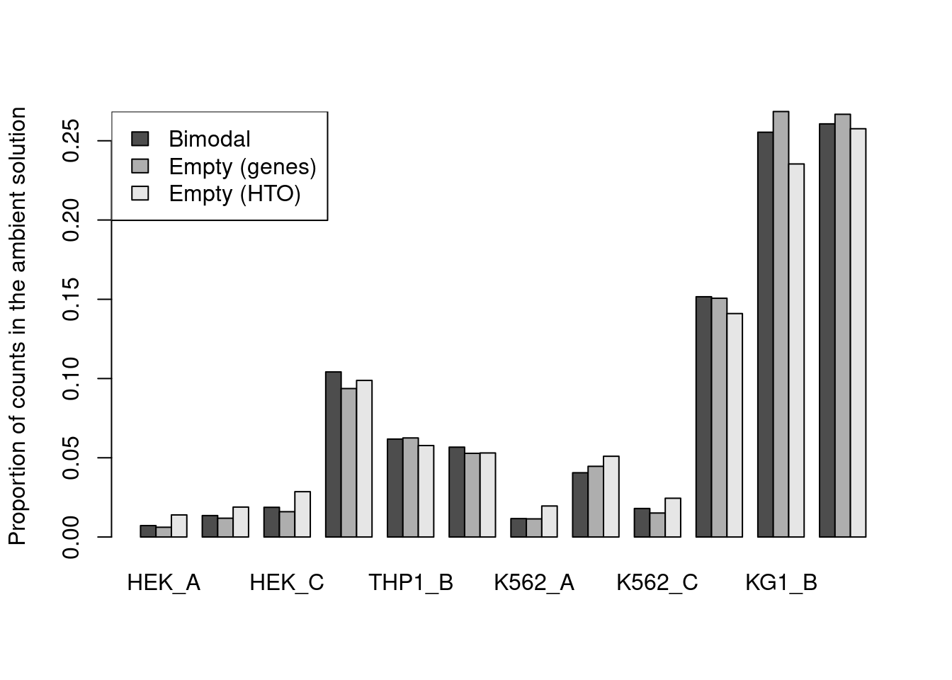
Figure 15.11: Proportion of each HTO in the ambient solution for the cell line mixture data, estimated using the bimodal method in hashedDrops() or by computing the average abundance across all empty droplets (where the empty state is defined by using emptyDrops() on either the genes or the HTO matrix).
Given an estimate of the ambient profile - say, the one derived from empty droplets detected using the HTO count matrix - we can easily use it in hashedDrops() via the ambient= argument.
This yields very similar results to those obtained with the automatic method, as expected from the similarity in the profiles.
hash.stats2 <- hashedDrops(hto.mat, ambient=metadata(e.out.hto)$ambient[,1])
table(hash.stats2$Best[hash.stats2$Confident])
##
## 1 2 3 4 5 6 7 8 9 10 11 12
## 575 602 565 526 551 559 354 598 411 632 553 58915.4.4 Further comments
After demultiplexing, it is a simple matter to subset the SingleCellExperiment to the confident assignments.
This actually involves two steps - the first is to subset to the libraries that were actually used in hashedDrops(), and the second is to subset to the libraries that were confidently assigned to a single sample.
Of course, we also include the putative sample of origin for each cell.
sce <- hto.sce[,rownames(hash.stats)]
sce$sample <- hash.stats$Best
sce <- sce[,hash.stats$Confident]
We examine the success of the demultiplexing by performing a quick analysis. Recall that this experiment involved 4 cell lines that were multiplexed together; we see that the separation between cell lines is preserved in Figure 15.12, indicating that the cells were assigned to their correct samples of origin.
library(scran)
library(scater)
sce <- logNormCounts(sce)
dec <- modelGeneVar(sce)

set.seed(100)
sce <- runPCA(sce, subset_row=getTopHVGs(dec, n=5000))
sce <- runTSNE(sce, dimred="PCA")

cell.lines <- sub("_.*", "", rownames(altExp(sce)))
sce$cell.line <- cell.lines[sce$sample]
plotTSNE(sce, colour_by="cell.line")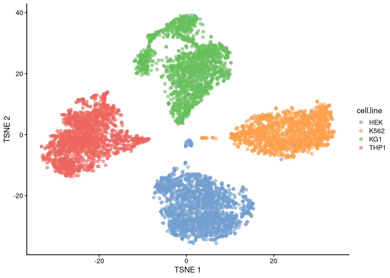
Figure 15.12: The usual \(t\)-SNE plot of the cell line mixture data, where each point is a cell and is colored by the cell line corresponding to its sample of origin.
Cell hashing information can also be used to detect doublets - see Chapter 16 for more details.
15.5 Removing swapped molecules
Some of the more recent DNA sequencing machines released by Illumina (e.g., HiSeq 3000/4000/X, X-Ten, and NovaSeq) use patterned flow cells to improve throughput and cost efficiency. However, in multiplexed pools, the use of these flow cells can lead to the mislabelling of DNA molecules with the incorrect library barcode (Sinha et al. 2017), a phenomenon known as “barcode swapping”. This leads to contamination of each library with reads from other libraries - for droplet sequencing experiments, this is particularly problematic as it manifests as the appearance of artificial cells that are low-coverage copies of their originals from other samples (Griffiths et al. 2018).
Fortunately, it is easy enough to remove affected reads from droplet experiments with the swappedDrops() function from DropletUtils.
Given a multiplexed pool of samples, we identify potential swapping events as transcript molecules that share the same combination of UMI sequence, assigned gene and cell barcode across samples.
We only keep the molecule if it has dominant coverage in a single sample, which is likely to be its original sample; we remove all (presumably swapped) instances of that molecule in the other samples.
Our assumption is that it is highly unlikely that two molecules would have the same combination of values by chance.
To demonstrate, we will use some multiplexed 10X Genomics data from an attempted study of the mouse mammary gland (Griffiths et al. 2018). This experiment consists of 8 scRNA-seq samples from various stages of mammary gland development, sequenced using the HiSeq 4000. We use the DropletTestFiles package to obtain the molecule information files produced by the CellRanger software suite; as its name suggests, this file format contains information on each individual transcript molecule in each sample.
library(DropletTestFiles)
swap.files <- listTestFiles(dataset="bach-mammary-swapping")
swap.files <- swap.files[dirname(swap.files$file.name)=="hiseq_4000",]
swap.files <- vapply(swap.files$rdatapath, getTestFile, prefix=FALSE, "")
names(swap.files) <- sub(".*_(.*)\\.h5", "\\1", names(swap.files))
We examine the barcode rank plots before making any attempt to remove swapped molecules (Figure 15.13), using the get10xMolInfoStats() function to efficiently obtain summary statistics from each molecule information file.
We see that samples E1 and F1 have different curves but this is not cause for alarm given that they also correspond to a different developmental stage compared to the other samples.
library(DropletUtils)
before.stats <- lapply(swap.files, get10xMolInfoStats)

max.umi <- vapply(before.stats, function(x) max(x$num.umis), 0)
ylim <- c(1, max(max.umi))
max.ncells <- vapply(before.stats, nrow, 0L)
xlim <- c(1, max(max.ncells))

plot(0,0,type="n", xlab="Rank", ylab="Number of UMIs",
    log="xy", xlim=xlim, ylim=ylim)
for (i in seq_along(before.stats)) {
    u <- sort(before.stats[[i]]$num.umis, decreasing=TRUE)
    lines(seq_along(u), u, col=i, lwd=5)
}

legend("topright", col=seq_along(before.stats),
    lwd=5, legend=names(before.stats))
Figure 15.13: Barcode rank curves for all samples in the HiSeq 4000-sequenced mammary gland dataset, before removing any swapped molecules.
We apply the swappedDrops() function to the molecule information files to identify and remove swapped molecules from each sample.
While all samples have some percentage of removed molecules, the majority of molecules in samples E1 and F1 are considered to be swapping artifacts.
The most likely cause is that these samples contain no real cells or highly damaged cells with little RNA, which frees up sequencing resources for deeper coverage of swapped molecules.
after.mat <- swappedDrops(swap.files, get.swapped=TRUE)
cleaned.sum <- vapply(after.mat$cleaned, sum, 0)
swapped.sum <- vapply(after.mat$swapped, sum, 0)
swapped.sum / (swapped.sum + cleaned.sum)
## A1 B1 C1 D1 E1 F1 G1 H1
## 0.02761 0.02767 0.12274 0.03797 0.82535 0.86561 0.02241 0.03648After removing the swapped molecules, the barcode rank curves for E1 and F1 drop dramatically (Figure 15.14). This represents the worst-case outcome of the swapping phenomenon, where cells are “carbon-copied”4 from the other multiplexed samples. Proceeding with the cleaned matrices protects us from these egregious artifacts as well as the more subtle effects of contamination.
plot(0,0,type="n", xlab="Rank", ylab="Number of UMIs",
    log="xy", xlim=xlim, ylim=ylim)

for (i in seq_along(after.mat$cleaned)) {
    cur.stats <- barcodeRanks(after.mat$cleaned[[i]])
    u <- sort(cur.stats$total, decreasing=TRUE)
    lines(seq_along(u), u, col=i, lwd=5)
}

legend("topright", col=seq_along(after.mat$cleaned),
    lwd=5, legend=names(after.mat$cleaned))
Figure 15.14: Barcode rank curves for all samples in the HiSeq 4000-sequenced mammary gland dataset, after removing any swapped molecules.
Session Info
R version 4.0.4 (2021-02-15)
Platform: x86_64-pc-linux-gnu (64-bit)
Running under: Ubuntu 20.04.2 LTS

Matrix products: default
BLAS:   /home/biocbuild/bbs-3.12-books/R/lib/libRblas.so
LAPACK: /home/biocbuild/bbs-3.12-books/R/lib/libRlapack.so

locale:
 [1] LC_CTYPE=en_US.UTF-8       LC_NUMERIC=C
 [3] LC_TIME=en_US.UTF-8        LC_COLLATE=C
 [5] LC_MONETARY=en_US.UTF-8    LC_MESSAGES=en_US.UTF-8
 [7] LC_PAPER=en_US.UTF-8       LC_NAME=C
 [9] LC_ADDRESS=C               LC_TELEPHONE=C
[11] LC_MEASUREMENT=en_US.UTF-8 LC_IDENTIFICATION=C

attached base packages:
[1] parallel  stats4    stats     graphics  grDevices utils     datasets
[8] methods   base

other attached packages:
 [1] DropletTestFiles_1.0.0      scran_1.18.5
 [3] scRNAseq_2.4.0              scater_1.18.6
 [5] ggplot2_3.3.3               scuttle_1.0.4
 [7] DropletUtils_1.10.3         SingleCellExperiment_1.12.0
 [9] SummarizedExperiment_1.20.0 Biobase_2.50.0
[11] GenomicRanges_1.42.0        GenomeInfoDb_1.26.4
[13] IRanges_2.24.1              S4Vectors_0.28.1
[15] BiocGenerics_0.36.0         MatrixGenerics_1.2.1
[17] matrixStats_0.58.0          BiocStyle_2.18.1
[19] rebook_1.0.0

loaded via a namespace (and not attached):
  [1] AnnotationHub_2.22.0          BiocFileCache_1.14.0
  [3] igraph_1.2.6                  lazyeval_0.2.2
  [5] BiocParallel_1.24.1           digest_0.6.27
  [7] ensembldb_2.14.0              htmltools_0.5.1.1
  [9] viridis_0.5.1                 fansi_0.4.2
 [11] magrittr_2.0.1                memoise_2.0.0
 [13] limma_3.46.0                  Biostrings_2.58.0
 [15] R.utils_2.10.1                askpass_1.1
 [17] prettyunits_1.1.1             colorspace_2.0-0
 [19] blob_1.2.1                    rappdirs_0.3.3
 [21] xfun_0.22                     dplyr_1.0.5
 [23] callr_3.5.1                   crayon_1.4.1
 [25] RCurl_1.98-1.3                jsonlite_1.7.2
 [27] graph_1.68.0                  glue_1.4.2
 [29] gtable_0.3.0                  zlibbioc_1.36.0
 [31] XVector_0.30.0                DelayedArray_0.16.2
 [33] BiocSingular_1.6.0            Rhdf5lib_1.12.1
 [35] HDF5Array_1.18.1              scales_1.1.1
 [37] DBI_1.1.1                     edgeR_3.32.1
 [39] Rcpp_1.0.6                    viridisLite_0.3.0
 [41] xtable_1.8-4                  progress_1.2.2
 [43] dqrng_0.2.1                   bit_4.0.4
 [45] rsvd_1.0.3                    httr_1.4.2
 [47] ellipsis_0.3.1                pkgconfig_2.0.3
 [49] XML_3.99-0.6                  R.methodsS3_1.8.1
 [51] farver_2.1.0                  CodeDepends_0.6.5
 [53] sass_0.3.1                    dbplyr_2.1.0
 [55] locfit_1.5-9.4                utf8_1.2.1
 [57] tidyselect_1.1.0              labeling_0.4.2
 [59] rlang_0.4.10                  later_1.1.0.1
 [61] AnnotationDbi_1.52.0          munsell_0.5.0
 [63] BiocVersion_3.12.0            tools_4.0.4
 [65] cachem_1.0.4                  generics_0.1.0
 [67] RSQLite_2.2.4                 ExperimentHub_1.16.0
 [69] evaluate_0.14                 stringr_1.4.0
 [71] fastmap_1.1.0                 yaml_2.2.1
 [73] processx_3.4.5                knitr_1.31
 [75] bit64_4.0.5                   purrr_0.3.4
 [77] AnnotationFilter_1.14.0       sparseMatrixStats_1.2.1
 [79] mime_0.10                     R.oo_1.24.0
 [81] xml2_1.3.2                    biomaRt_2.46.3
 [83] compiler_4.0.4                beeswarm_0.3.1
 [85] curl_4.3                      interactiveDisplayBase_1.28.0
 [87] statmod_1.4.35                tibble_3.1.0
 [89] bslib_0.2.4                   stringi_1.5.3
 [91] highr_0.8                     ps_1.6.0
 [93] GenomicFeatures_1.42.2        bluster_1.0.0
 [95] lattice_0.20-41               ProtGenerics_1.22.0
 [97] Matrix_1.3-2                  vctrs_0.3.6
 [99] pillar_1.5.1                  lifecycle_1.0.0
[101] rhdf5filters_1.2.0            BiocManager_1.30.10
[103] jquerylib_0.1.3               BiocNeighbors_1.8.2
[105] cowplot_1.1.1                 bitops_1.0-6
[107] irlba_2.3.3                   rtracklayer_1.50.0
[109] httpuv_1.5.5                  R6_2.5.0
[111] bookdown_0.21                 promises_1.2.0.1
[113] gridExtra_2.3                 vipor_0.4.5
[115] codetools_0.2-18              assertthat_0.2.1
[117] rhdf5_2.34.0                  openssl_1.4.3
[119] withr_2.4.1                   GenomicAlignments_1.26.0
[121] Rsamtools_2.6.0               GenomeInfoDbData_1.2.4
[123] hms_1.0.0                     grid_4.0.4
[125] beachmat_2.6.4                rmarkdown_2.7
[127] DelayedMatrixStats_1.12.3     Rtsne_0.15
[129] shiny_1.6.0                   ggbeeswarm_0.6.0
Bibliography
Griffiths, J. A., A. C. Richard, K. Bach, A. T. L. Lun, and J. C. Marioni. 2018. “Detection and removal of barcode swapping in single-cell RNA-seq data.” Nat Commun 9 (1): 2667.
Klein, A. M., L. Mazutis, I. Akartuna, N. Tallapragada, A. Veres, V. Li, L. Peshkin, D. A. Weitz, and M. W. Kirschner. 2015. “Droplet barcoding for single-cell transcriptomics applied to embryonic stem cells.” Cell 161 (5): 1187–1201.
Lun, A., S. Riesenfeld, T. Andrews, T. P. Dao, T. Gomes, participants in the 1st Human Cell Atlas Jamboree, and J. Marioni. 2019. “EmptyDrops: distinguishing cells from empty droplets in droplet-based single-cell RNA sequencing data.” Genome Biol. 20 (1): 63.
Macosko, E. Z., A. Basu, R. Satija, J. Nemesh, K. Shekhar, M. Goldman, I. Tirosh, et al. 2015. “Highly parallel genome-wide expression profiling of individual cells using nanoliter droplets.” Cell 161 (5): 1202–14.
McGinnis, C. S., D. M. Patterson, J. Winkler, D. N. Conrad, M. Y. Hein, V. Srivastava, J. L. Hu, et al. 2019. “MULTI-seq: sample multiplexing for single-cell RNA sequencing using lipid-tagged indices.” Nat. Methods 16 (7): 619–26.
Phipson, B., and G. K. Smyth. 2010. “Permutation P-values should never be zero: calculating exact P-values when permutations are randomly drawn.” Stat. Appl. Genet. Mol. Biol. 9: Article 39.
Sinha, Rahul, Geoff Stanley, Gunsagar S. Gulati, Camille Ezran, Kyle J. Travaglini, Eric Wei, Charles K.F. Chan, et al. 2017. “Index Switching Causes “Spreading-of-Signal” Among Multiplexed Samples in Illumina Hiseq 4000 Dna Sequencing.” bioRxiv. https://doi.org/10.1101/125724.
Stoeckius, M., S. Zheng, B. Houck-Loomis, S. Hao, B. Z. Yeung, W. M. Mauck, P. Smibert, and R. Satija. 2018. “Cell Hashing with barcoded antibodies enables multiplexing and doublet detection for single cell genomics.” Genome Biol. 19 (1): 224.
Young, M. D., and S. Behjati. 2018. “SoupX Removes Ambient RNA Contamination from Droplet Based Single Cell RNA Sequencing Data.” bioRxiv.
Zheng, G. X., J. M. Terry, P. Belgrader, P. Ryvkin, Z. W. Bent, R. Wilson, S. B. Ziraldo, et al. 2017. “Massively parallel digital transcriptional profiling of single cells.” Nat Commun 8 (January): 14049.