Chapter 38 Merged mouse HSC datasets
38.1 Introduction
The blood is probably the most well-studied tissue in the single-cell field, mostly because everything is already dissociated “for free”. Of particular interest has been the use of single-cell genomics to study cell fate decisions in haematopoeisis. Indeed, it was not long ago that dueling interpretations of haematopoeitic stem cell (HSC) datasets were a mainstay of single-cell conferences. Sadly, these times have mostly passed so we will instead entertain ourselves by combining a small number of these datasets into a single analysis.
38.2 Data loading
#--- data-loading ---#
library(scRNAseq)
sce.nest <- NestorowaHSCData()

#--- gene-annotation ---#
library(AnnotationHub)
ens.mm.v97 <- AnnotationHub()[["AH73905"]]
anno <- select(ens.mm.v97, keys=rownames(sce.nest),
    keytype="GENEID", columns=c("SYMBOL", "SEQNAME"))
rowData(sce.nest) <- anno[match(rownames(sce.nest), anno$GENEID),]

#--- quality-control-grun ---#
library(scater)
stats <- perCellQCMetrics(sce.nest)
qc <- quickPerCellQC(stats, percent_subsets="altexps_ERCC_percent")
sce.nest <- sce.nest[,!qc$discard]

#--- normalization ---#
library(scran)
set.seed(101000110)
clusters <- quickCluster(sce.nest)
sce.nest <- computeSumFactors(sce.nest, clusters=clusters)
sce.nest <- logNormCounts(sce.nest)

#--- variance-modelling ---#
set.seed(00010101)
dec.nest <- modelGeneVarWithSpikes(sce.nest, "ERCC")
top.nest <- getTopHVGs(dec.nest, prop=0.1)## class: SingleCellExperiment
## dim: 46078 1656
## metadata(0):
## assays(2): counts logcounts
## rownames(46078): ENSMUSG00000000001 ENSMUSG00000000003 ...
## ENSMUSG00000107391 ENSMUSG00000107392
## rowData names(3): GENEID SYMBOL SEQNAME
## colnames(1656): HSPC_025 HSPC_031 ... Prog_852 Prog_810
## colData names(3): cell.type FACS sizeFactor
## reducedDimNames(1): diffusion
## altExpNames(1): ERCCThe Grun dataset requires a little bit of subsetting and re-analysis to only consider the sorted HSCs.
#--- data-loading ---#
library(scRNAseq)
sce.grun.hsc <- GrunHSCData(ensembl=TRUE)

#--- gene-annotation ---#
library(AnnotationHub)
ens.mm.v97 <- AnnotationHub()[["AH73905"]]
anno <- select(ens.mm.v97, keys=rownames(sce.grun.hsc),
    keytype="GENEID", columns=c("SYMBOL", "SEQNAME"))
rowData(sce.grun.hsc) <- anno[match(rownames(sce.grun.hsc), anno$GENEID),]

#--- quality-control ---#
library(scuttle)
stats <- perCellQCMetrics(sce.grun.hsc)
qc <- quickPerCellQC(stats, batch=sce.grun.hsc$protocol,
    subset=grepl("sorted", sce.grun.hsc$protocol))
sce.grun.hsc <- sce.grun.hsc[,!qc$discard]library(scuttle)
sce.grun.hsc <- sce.grun.hsc[,sce.grun.hsc$protocol=="sorted hematopoietic stem cells"]
sce.grun.hsc <- logNormCounts(sce.grun.hsc)
set.seed(11001)
library(scran)
dec.grun.hsc <- modelGeneVarByPoisson(sce.grun.hsc) Finally, we will grab the Paul dataset, which we will also subset to only consider the unsorted myeloid population. This removes the various knockout conditions that just complicates matters.
#--- data-loading ---#
library(scRNAseq)
sce.paul <- PaulHSCData(ensembl=TRUE)

#--- gene-annotation ---#
library(AnnotationHub)
ens.mm.v97 <- AnnotationHub()[["AH73905"]]
anno <- select(ens.mm.v97, keys=rownames(sce.paul),
    keytype="GENEID", columns=c("SYMBOL", "SEQNAME"))
rowData(sce.paul) <- anno[match(rownames(sce.paul), anno$GENEID),]

#--- quality-control ---#
library(scater)
stats <- perCellQCMetrics(sce.paul)
qc <- quickPerCellQC(stats, batch=sce.paul$Plate_ID)

# Detecting batches with unusually low threshold values.
lib.thresholds <- attr(qc$low_lib_size, "thresholds")["lower",]
nfeat.thresholds <- attr(qc$low_n_features, "thresholds")["lower",]
ignore <- union(names(lib.thresholds)[lib.thresholds < 100],
    names(nfeat.thresholds)[nfeat.thresholds < 100])

# Repeating the QC using only the "high-quality" batches.
qc2 <- quickPerCellQC(stats, batch=sce.paul$Plate_ID,
    subset=!sce.paul$Plate_ID %in% ignore)
sce.paul <- sce.paul[,!qc2$discard]38.3 Setting up the merge
common <- Reduce(intersect, list(rownames(sce.nest),
    rownames(sce.grun.hsc), rownames(sce.paul)))
length(common)
## [1] 17147Combining variances to obtain a single set of HVGs.
combined.dec <- combineVar(
    dec.nest[common,],
    dec.grun.hsc[common,],
    dec.paul[common,]
)
hvgs <- getTopHVGs(combined.dec, n=5000)
Adjusting for gross differences in sequencing depth.
38.4 Merging the datasets
We turn on auto.merge=TRUE to instruct fastMNN() to merge the batch that offers the largest number of MNNs.
This aims to perform the “easiest” merges first, i.e., between the most replicate-like batches,
before tackling merges between batches that have greater differences in their population composition.
Not too much variance lost inside each batch, hopefully. We also observe that the algorithm chose to merge the more diverse Nestorowa and Paul datasets before dealing with the HSC-only Grun dataset.
## DataFrame with 2 rows and 3 columns
##             left     right                        lost.var
##           <List>    <List>                        <matrix>
## 1           Paul Nestorowa 0.01069374:0.0000000:0.00739465
## 2 Paul,Nestorowa      Grun 0.00562344:0.0178334:0.00702615
38.5 Combined analyses
The Grun dataset does not contribute to many clusters, consistent with a pure undifferentiated HSC population. Most of the other clusters contain contributions from the Nestorowa and Paul datasets, though some are unique to the Paul dataset. This may be due to incomplete correction though we tend to think that this are Paul-specific subpopulations, given that the Nestorowa dataset does not have similarly sized unique clusters that might represent their uncorrected counterparts.
library(bluster)
colLabels(merged) <- clusterRows(reducedDim(merged),
    NNGraphParam(cluster.fun="louvain"))
table(Cluster=colLabels(merged), Batch=merged$batch)
## Batch
## Cluster Grun Nestorowa Paul
## 1 0 40 206
## 2 0 19 0
## 3 39 353 146
## 4 0 6 29
## 5 0 217 487
## 6 0 162 522
## 7 0 133 191
## 8 22 411 94
## 9 230 315 348
## 10 0 0 385
## 11 0 0 397While I prefer \(t\)-SNE plots, we’ll switch to a UMAP plot to highlight some of the trajectory-like structure across clusters (Figure 38.1).
library(scater)
set.seed(101010101)
merged <- runUMAP(merged, dimred="corrected")
gridExtra::grid.arrange(
    plotUMAP(merged, colour_by="label"),
    plotUMAP(merged, colour_by="batch"),
    ncol=2
)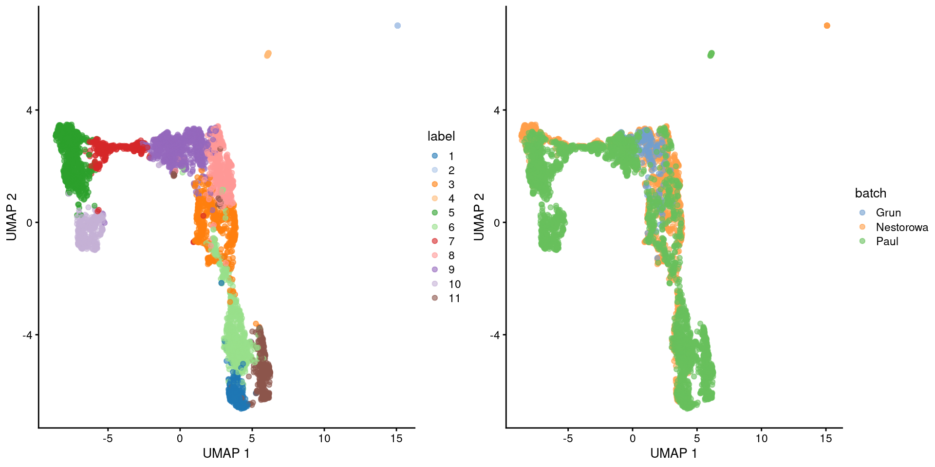
Figure 38.1: Obligatory UMAP plot of the merged HSC datasets, where each point represents a cell and is colored by the batch of origin (left) or its assigned cluster (right).
In fact, we might as well compute a trajectory right now. TSCAN constructs a reasonable minimum spanning tree but the path choices are somewhat incongruent with the UMAP coordinates (Figure 38.2). This is most likely due to the fact that TSCAN operates on cluster centroids, which is simple and efficient but does not consider the variance of cells within each cluster. It is entirely possible for two well-separated clusters to be closer than two adjacent clusters if the latter span a wider region of the coordinate space.
common.pseudo <- rowMeans(pseudo.out$ordering, na.rm=TRUE)
plotUMAP(merged, colour_by=I(common.pseudo),
        text_by="label", text_colour="red") +
    geom_line(data=pseudo.out$connected$UMAP,
        mapping=aes(x=dim1, y=dim2, group=edge))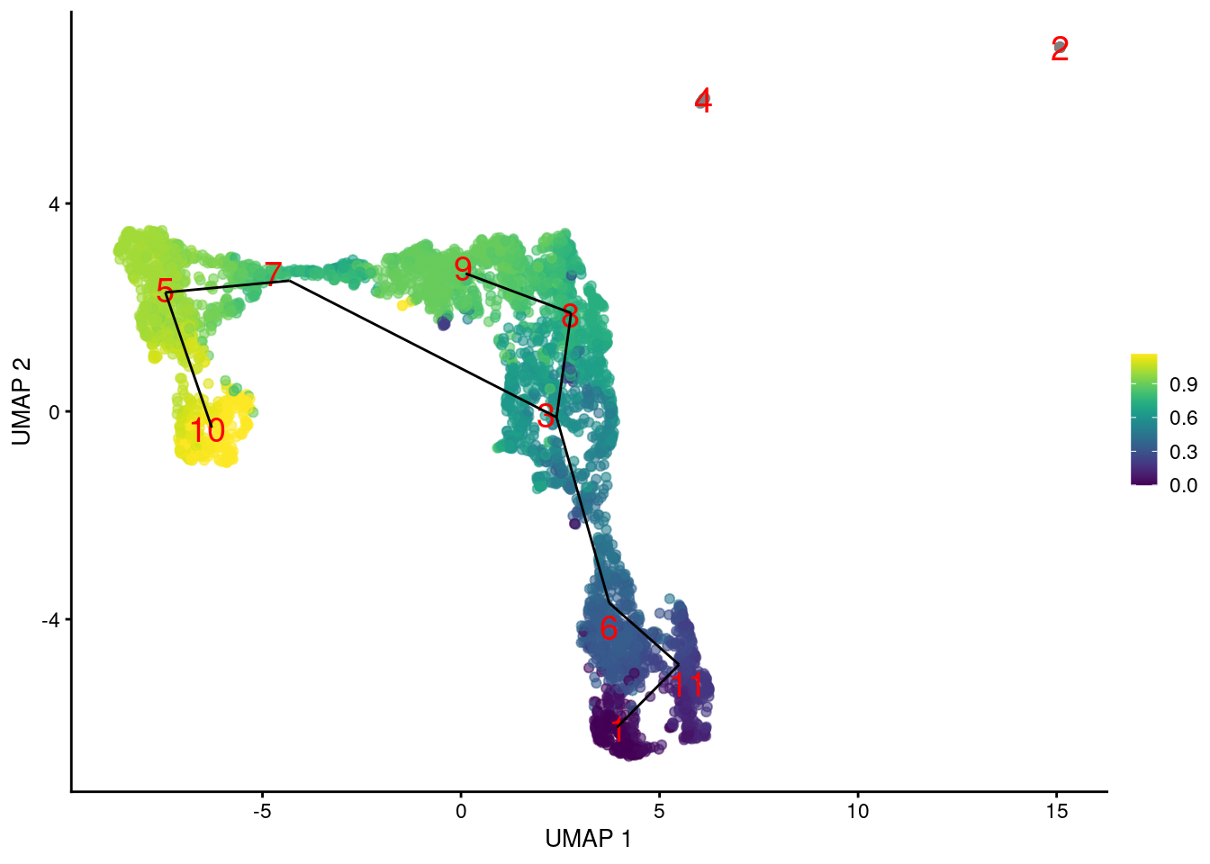
Figure 38.2: Another UMAP plot of the merged HSC datasets, where each point represents a cell and is colored by its TSCAN pseudotime. The lines correspond to the edges of the MST across cluster centers.
To fix this, we construct the minimum spanning tree using distances based on pairs of mutual nearest neighbors between clusters. This focuses on the closeness of the boundaries of each pair of clusters rather than their centroids, ensuring that adjacent clusters are connected even if their centroids are far apart. Doing so yields a trajectory that is more consistent with the visual connections on the UMAP plot (Figure 38.3).
pseudo.out2 <- quickPseudotime(merged, use.dimred="corrected",
    with.mnn=TRUE, outgroup=TRUE)

common.pseudo2 <- rowMeans(pseudo.out2$ordering, na.rm=TRUE)
plotUMAP(merged, colour_by=I(common.pseudo2),
        text_by="label", text_colour="red") +
    geom_line(data=pseudo.out2$connected$UMAP,
        mapping=aes(x=dim1, y=dim2, group=edge))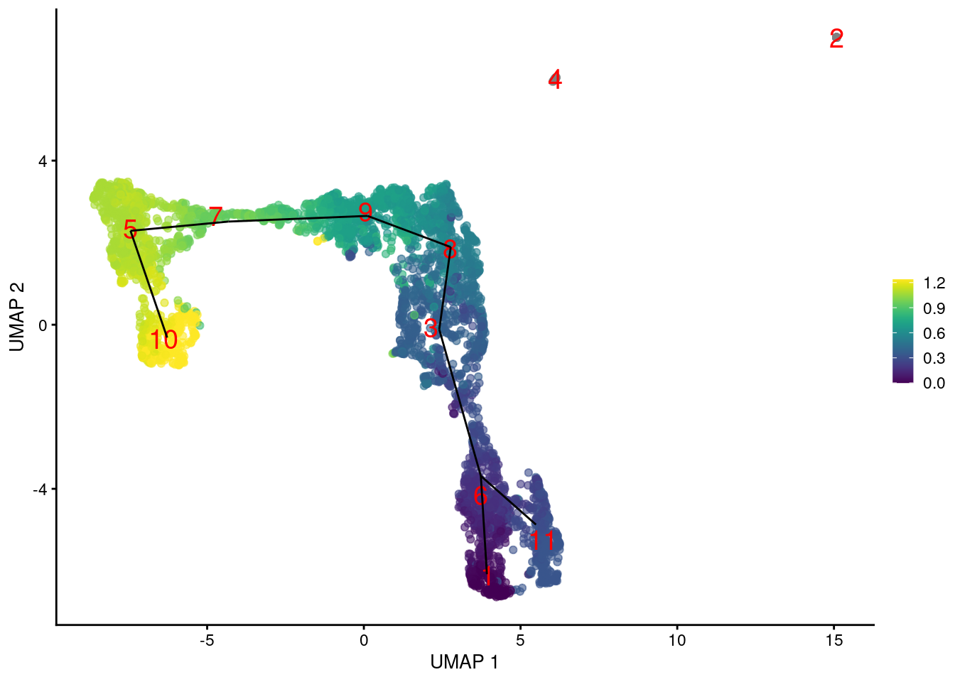
Figure 38.3: Yet another UMAP plot of the merged HSC datasets, where each point represents a cell and is colored by its TSCAN pseudotime. The lines correspond to the edges of the MST across cluster centers.
Session Info
R version 4.0.4 (2021-02-15)
Platform: x86_64-pc-linux-gnu (64-bit)
Running under: Ubuntu 20.04.2 LTS

Matrix products: default
BLAS:   /home/biocbuild/bbs-3.12-books/R/lib/libRblas.so
LAPACK: /home/biocbuild/bbs-3.12-books/R/lib/libRlapack.so

locale:
 [1] LC_CTYPE=en_US.UTF-8       LC_NUMERIC=C
 [3] LC_TIME=en_US.UTF-8        LC_COLLATE=C
 [5] LC_MONETARY=en_US.UTF-8    LC_MESSAGES=en_US.UTF-8
 [7] LC_PAPER=en_US.UTF-8       LC_NAME=C
 [9] LC_ADDRESS=C               LC_TELEPHONE=C
[11] LC_MEASUREMENT=en_US.UTF-8 LC_IDENTIFICATION=C

attached base packages:
[1] parallel  stats4    stats     graphics  grDevices utils     datasets
[8] methods   base

other attached packages:
 [1] TSCAN_1.28.0                scater_1.18.6
 [3] ggplot2_3.3.3               bluster_1.0.0
 [5] batchelor_1.6.2             scran_1.18.5
 [7] scuttle_1.0.4               SingleCellExperiment_1.12.0
 [9] SummarizedExperiment_1.20.0 Biobase_2.50.0
[11] GenomicRanges_1.42.0        GenomeInfoDb_1.26.4
[13] IRanges_2.24.1              S4Vectors_0.28.1
[15] BiocGenerics_0.36.0         MatrixGenerics_1.2.1
[17] matrixStats_0.58.0          BiocStyle_2.18.1
[19] rebook_1.0.0

loaded via a namespace (and not attached):
  [1] ggbeeswarm_0.6.0          colorspace_2.0-0
  [3] ellipsis_0.3.1            mclust_5.4.7
  [5] XVector_0.30.0            BiocNeighbors_1.8.2
  [7] farver_2.1.0              fansi_0.4.2
  [9] codetools_0.2-18          splines_4.0.4
 [11] sparseMatrixStats_1.2.1   knitr_1.31
 [13] jsonlite_1.7.2            ResidualMatrix_1.0.0
 [15] graph_1.68.0              uwot_0.1.10
 [17] shiny_1.6.0               BiocManager_1.30.10
 [19] compiler_4.0.4            dqrng_0.2.1
 [21] fastmap_1.1.0             assertthat_0.2.1
 [23] Matrix_1.3-2              limma_3.46.0
 [25] later_1.1.0.1             BiocSingular_1.6.0
 [27] htmltools_0.5.1.1         tools_4.0.4
 [29] rsvd_1.0.3                igraph_1.2.6
 [31] gtable_0.3.0              glue_1.4.2
 [33] GenomeInfoDbData_1.2.4    dplyr_1.0.5
 [35] Rcpp_1.0.6                jquerylib_0.1.3
 [37] vctrs_0.3.6               nlme_3.1-152
 [39] DelayedMatrixStats_1.12.3 xfun_0.22
 [41] stringr_1.4.0             ps_1.6.0
 [43] beachmat_2.6.4            mime_0.10
 [45] lifecycle_1.0.0           irlba_2.3.3
 [47] gtools_3.8.2              statmod_1.4.35
 [49] XML_3.99-0.6              edgeR_3.32.1
 [51] zlibbioc_1.36.0           scales_1.1.1
 [53] promises_1.2.0.1          yaml_2.2.1
 [55] gridExtra_2.3             sass_0.3.1
 [57] fastICA_1.2-2             stringi_1.5.3
 [59] highr_0.8                 caTools_1.18.1
 [61] BiocParallel_1.24.1       rlang_0.4.10
 [63] pkgconfig_2.0.3           bitops_1.0-6
 [65] evaluate_0.14             lattice_0.20-41
 [67] purrr_0.3.4               CodeDepends_0.6.5
 [69] labeling_0.4.2            cowplot_1.1.1
 [71] processx_3.4.5            tidyselect_1.1.0
 [73] RcppAnnoy_0.0.18          plyr_1.8.6
 [75] magrittr_2.0.1            bookdown_0.21
 [77] R6_2.5.0                  gplots_3.1.1
 [79] generics_0.1.0            combinat_0.0-8
 [81] DelayedArray_0.16.2       DBI_1.1.1
 [83] pillar_1.5.1              withr_2.4.1
 [85] mgcv_1.8-33               RCurl_1.98-1.3
 [87] tibble_3.1.0              crayon_1.4.1
 [89] KernSmooth_2.23-18        utf8_1.2.1
 [91] rmarkdown_2.7             viridis_0.5.1
 [93] locfit_1.5-9.4            grid_4.0.4
 [95] callr_3.5.1               digest_0.6.27
 [97] xtable_1.8-4              httpuv_1.5.5
 [99] munsell_0.5.0             beeswarm_0.3.1
[101] viridisLite_0.3.0         vipor_0.4.5
[103] bslib_0.2.4