Chapter 34 Merged human pancreas datasets
34.1 Introduction
For a period in 2016, there was a great deal of interest in using scRNA-seq to profile the human pancreas at cellular resolution (Muraro et al. 2016; Grun et al. 2016; Lawlor et al. 2017; Segerstolpe et al. 2016). As a consequence, we have a surplus of human pancreas datasets generated by different authors with different technologies, which provides an ideal use case for demonstrating more complex data integration strategies. This represents a more challenging application than the PBMC dataset in Chapter 13 as it involves different sequencing protocols and different patients, most likely with differences in cell type composition.
34.2 The good
We start by considering only two datasets from Muraro et al. (2016) and Grun et al. (2016). This is a relatively simple scenario involving very similar protocols (CEL-seq and CEL-seq2) and a similar set of authors.
#--- loading ---#
library(scRNAseq)
sce.grun <- GrunPancreasData()

#--- gene-annotation ---#
library(org.Hs.eg.db)
gene.ids <- mapIds(org.Hs.eg.db, keys=rowData(sce.grun)$symbol,
    keytype="SYMBOL", column="ENSEMBL")

keep <- !is.na(gene.ids) & !duplicated(gene.ids)
sce.grun <- sce.grun[keep,]
rownames(sce.grun) <- gene.ids[keep]

#--- quality-control ---#
library(scater)
stats <- perCellQCMetrics(sce.grun)

qc <- quickPerCellQC(stats, percent_subsets="altexps_ERCC_percent",
    batch=sce.grun$donor,
    subset=sce.grun$donor %in% c("D17", "D7", "D2"))

sce.grun <- sce.grun[,!qc$discard]

#--- normalization ---#
library(scran)
set.seed(1000) # for irlba.
clusters <- quickCluster(sce.grun)
sce.grun <- computeSumFactors(sce.grun, clusters=clusters)
sce.grun <- logNormCounts(sce.grun)

#--- variance-modelling ---#
block <- paste0(sce.grun$sample, "_", sce.grun$donor)
dec.grun <- modelGeneVarWithSpikes(sce.grun, spikes="ERCC", block=block)
top.grun <- getTopHVGs(dec.grun, prop=0.1)## class: SingleCellExperiment
## dim: 17474 1063
## metadata(0):
## assays(2): counts logcounts
## rownames(17474): ENSG00000268895 ENSG00000121410 ... ENSG00000074755
## ENSG00000036549
## rowData names(2): symbol chr
## colnames(1063): D2ex_1 D2ex_2 ... D17TGFB_94 D17TGFB_95
## colData names(3): donor sample sizeFactor
## reducedDimNames(0):
## altExpNames(1): ERCC#--- loading ---#
library(scRNAseq)
sce.muraro <- MuraroPancreasData()
#--- gene-annotation ---#
library(AnnotationHub)
edb <- AnnotationHub()[["AH73881"]]
gene.symb <- sub("__chr.*$", "", rownames(sce.muraro))
gene.ids <- mapIds(edb, keys=gene.symb,
keytype="SYMBOL", column="GENEID")
# Removing duplicated genes or genes without Ensembl IDs.
keep <- !is.na(gene.ids) & !duplicated(gene.ids)
sce.muraro <- sce.muraro[keep,]
rownames(sce.muraro) <- gene.ids[keep]
#--- quality-control ---#
library(scater)
stats <- perCellQCMetrics(sce.muraro)
qc <- quickPerCellQC(stats, percent_subsets="altexps_ERCC_percent",
batch=sce.muraro$donor, subset=sce.muraro$donor!="D28")
sce.muraro <- sce.muraro[,!qc$discard]
#--- normalization ---#
library(scran)
set.seed(1000)
clusters <- quickCluster(sce.muraro)
sce.muraro <- computeSumFactors(sce.muraro, clusters=clusters)
sce.muraro <- logNormCounts(sce.muraro)
#--- variance-modelling ---#
block <- paste0(sce.muraro$plate, "_", sce.muraro$donor)
dec.muraro <- modelGeneVarWithSpikes(sce.muraro, "ERCC", block=block)
top.muraro <- getTopHVGs(dec.muraro, prop=0.1)## class: SingleCellExperiment
## dim: 16940 2299
## metadata(0):
## assays(2): counts logcounts
## rownames(16940): ENSG00000268895 ENSG00000121410 ... ENSG00000159840
## ENSG00000074755
## rowData names(2): symbol chr
## colnames(2299): D28-1_1 D28-1_2 ... D30-8_93 D30-8_94
## colData names(4): label donor plate sizeFactor
## reducedDimNames(0):
## altExpNames(1): ERCCWe subset both batches to their common universe of genes; adjust their scaling to equalize sequencing coverage (not really necessary in this case, as the coverage is already similar, but we will do so anyway for consistency); and select those genes with positive average biological components for further use.
universe <- intersect(rownames(sce.grun), rownames(sce.muraro))
sce.grun2 <- sce.grun[universe,]
dec.grun2 <- dec.grun[universe,]
sce.muraro2 <- sce.muraro[universe,]
dec.muraro2 <- dec.muraro[universe,]

library(batchelor)
normed.pancreas <- multiBatchNorm(sce.grun2, sce.muraro2)
sce.grun2 <- normed.pancreas[[1]]
sce.muraro2 <- normed.pancreas[[2]]

library(scran)
combined.pan <- combineVar(dec.grun2, dec.muraro2)
chosen.genes <- rownames(combined.pan)[combined.pan$bio > 0]
We observe that rescaleBatches() is unable to align cells from different batches in Figure 34.1.
This is attributable to differences in population composition between batches, with additional complications from non-linearities in the batch effect, e.g., when the magnitude or direction of the batch effect differs between cell types.
library(scater)
rescaled.pancreas <- rescaleBatches(sce.grun2, sce.muraro2)

set.seed(100101)
rescaled.pancreas <- runPCA(rescaled.pancreas, subset_row=chosen.genes,
    exprs_values="corrected")

rescaled.pancreas <- runTSNE(rescaled.pancreas, dimred="PCA")
plotTSNE(rescaled.pancreas, colour_by="batch")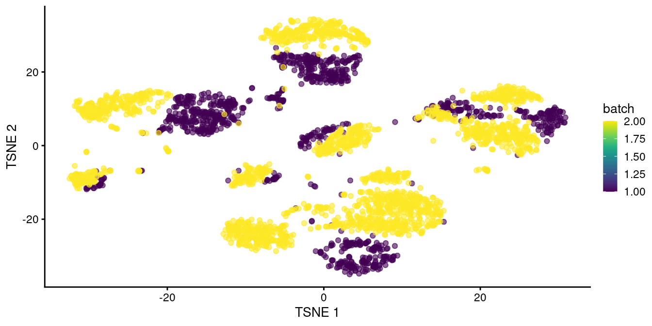
Figure 34.1: \(t\)-SNE plot of the two pancreas datasets after correction with rescaleBatches(). Each point represents a cell and is colored according to the batch of origin.
Here, we use fastMNN() to merge together the two human pancreas datasets described earlier.
Clustering on the merged datasets yields fewer batch-specific clusters, which is recapitulated as greater intermingling between batches in Figure 34.2.
This improvement over Figure 34.1 represents the ability of fastMNN() to adapt to more complex situations involving differences in population composition between batches.
set.seed(1011011)
mnn.pancreas <- fastMNN(sce.grun2, sce.muraro2, subset.row=chosen.genes)

snn.gr <- buildSNNGraph(mnn.pancreas, use.dimred="corrected")
clusters <- igraph::cluster_walktrap(snn.gr)$membership
tab <- table(Cluster=clusters, Batch=mnn.pancreas$batch)
tab
## Batch
## Cluster 1 2
## 1 243 280
## 2 315 255
## 3 203 843
## 4 56 194
## 5 24 108
## 6 116 398
## 7 27 0
## 8 56 72
## 9 18 113
## 10 0 17
## 11 5 19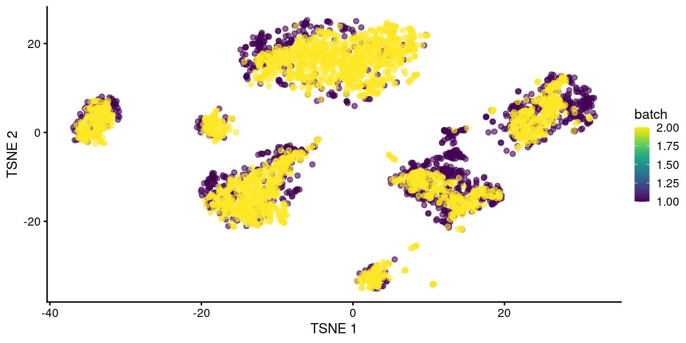
Figure 34.2: \(t\)-SNE plot of the two pancreas datasets after correction with fastMNN(). Each point represents a cell and is colored according to the batch of origin.
34.3 The bad
Flushed with our previous success, we now attempt to merge the other datasets from Lawlor et al. (2017) and Segerstolpe et al. (2016). This is a more challenging task as it involves different technologies, mixtures of UMI and read count data and a more diverse set of authors (presumably with greater differences in the patient population).
#--- loading ---#
library(scRNAseq)
sce.lawlor <- LawlorPancreasData()

#--- gene-annotation ---#
library(AnnotationHub)
edb <- AnnotationHub()[["AH73881"]]
anno <- select(edb, keys=rownames(sce.lawlor), keytype="GENEID",
    columns=c("SYMBOL", "SEQNAME"))
rowData(sce.lawlor) <- anno[match(rownames(sce.lawlor), anno[,1]),-1]

#--- quality-control ---#
library(scater)
stats <- perCellQCMetrics(sce.lawlor,
    subsets=list(Mito=which(rowData(sce.lawlor)$SEQNAME=="MT")))
qc <- quickPerCellQC(stats, percent_subsets="subsets_Mito_percent",
    batch=sce.lawlor$`islet unos id`)
sce.lawlor <- sce.lawlor[,!qc$discard]

#--- normalization ---#
library(scran)
set.seed(1000)
clusters <- quickCluster(sce.lawlor)
sce.lawlor <- computeSumFactors(sce.lawlor, clusters=clusters)
sce.lawlor <- logNormCounts(sce.lawlor)

#--- variance-modelling ---#
dec.lawlor <- modelGeneVar(sce.lawlor, block=sce.lawlor$`islet unos id`)
chosen.genes <- getTopHVGs(dec.lawlor, n=2000)## class: SingleCellExperiment
## dim: 26616 604
## metadata(0):
## assays(2): counts logcounts
## rownames(26616): ENSG00000229483 ENSG00000232849 ... ENSG00000251576
## ENSG00000082898
## rowData names(2): SYMBOL SEQNAME
## colnames(604): 10th_C11_S96 10th_C13_S61 ... 9th-C96_S81 9th-C9_S13
## colData names(9): title age ... Sex sizeFactor
## reducedDimNames(0):
## altExpNames(0):#--- loading ---#
library(scRNAseq)
sce.seger <- SegerstolpePancreasData()
#--- gene-annotation ---#
library(AnnotationHub)
edb <- AnnotationHub()[["AH73881"]]
symbols <- rowData(sce.seger)$symbol
ens.id <- mapIds(edb, keys=symbols, keytype="SYMBOL", column="GENEID")
ens.id <- ifelse(is.na(ens.id), symbols, ens.id)
# Removing duplicated rows.
keep <- !duplicated(ens.id)
sce.seger <- sce.seger[keep,]
rownames(sce.seger) <- ens.id[keep]
#--- sample-annotation ---#
emtab.meta <- colData(sce.seger)[,c("cell type", "disease",
"individual", "single cell well quality")]
colnames(emtab.meta) <- c("CellType", "Disease", "Donor", "Quality")
colData(sce.seger) <- emtab.meta
sce.seger$CellType <- gsub(" cell", "", sce.seger$CellType)
sce.seger$CellType <- paste0(
toupper(substr(sce.seger$CellType, 1, 1)),
substring(sce.seger$CellType, 2))
#--- quality-control ---#
low.qual <- sce.seger$Quality == "low quality cell"
library(scater)
stats <- perCellQCMetrics(sce.seger)
qc <- quickPerCellQC(stats, percent_subsets="altexps_ERCC_percent",
batch=sce.seger$Donor,
subset=!sce.seger$Donor %in% c("HP1504901", "HP1509101"))
sce.seger <- sce.seger[,!(qc$discard | low.qual)]
#--- normalization ---#
library(scran)
clusters <- quickCluster(sce.seger)
sce.seger <- computeSumFactors(sce.seger, clusters=clusters)
sce.seger <- logNormCounts(sce.seger)
#--- variance-modelling ---#
for.hvg <- sce.seger[,librarySizeFactors(altExp(sce.seger)) > 0 & sce.seger$Donor!="AZ"]
dec.seger <- modelGeneVarWithSpikes(for.hvg, "ERCC", block=for.hvg$Donor)
chosen.hvgs <- getTopHVGs(dec.seger, n=2000)## class: SingleCellExperiment
## dim: 25454 2090
## metadata(0):
## assays(2): counts logcounts
## rownames(25454): ENSG00000118473 ENSG00000142920 ... ENSG00000278306
## eGFP
## rowData names(2): symbol refseq
## colnames(2090): HP1502401_H13 HP1502401_J14 ... HP1526901T2D_N8
## HP1526901T2D_A8
## colData names(5): CellType Disease Donor Quality sizeFactor
## reducedDimNames(0):
## altExpNames(1): ERCCWe perform the usual routine to obtain re-normalized values and a set of HVGs. Here, we put all the objects into a list to avoid having to explicitly type their names separately.
all.sce <- list(Grun=sce.grun, Muraro=sce.muraro,
    Lawlor=sce.lawlor, Seger=sce.seger)
all.dec <- list(Grun=dec.grun, Muraro=dec.muraro,
    Lawlor=dec.lawlor, Seger=dec.seger)

universe <- Reduce(intersect, lapply(all.sce, rownames))
all.sce <- lapply(all.sce, "[", i=universe,)
all.dec <- lapply(all.dec, "[", i=universe,)

normed.pancreas <- do.call(multiBatchNorm, all.sce)
combined.pan <- do.call(combineVar, all.dec)
chosen.genes <- rownames(combined.pan)[combined.pan$bio > 0]
We observe that the merge is generally successful, with many clusters containing contributions from each batch (Figure 34.3). There are few clusters that are specific to the Segerstolpe dataset, and if we were naive, we might consider them to represent interesting subpopulations that are not present in the other datasets.
set.seed(1011110)
mnn.pancreas <- fastMNN(normed.pancreas)

# Bumping up 'k' to get broader clusters for this demonstration.
snn.gr <- buildSNNGraph(mnn.pancreas, use.dimred="corrected", k=20)
clusters <- igraph::cluster_walktrap(snn.gr)$membership
clusters <- factor(clusters)
tab <- table(Cluster=clusters, Batch=mnn.pancreas$batch)
tab
## Batch
## Cluster Grun Lawlor Muraro Seger
## 1 304 28 256 383
## 2 103 244 382 174
## 3 0 0 0 55
## 4 219 16 241 140
## 5 166 231 357 149
## 6 34 0 1 0
## 7 56 17 196 109
## 8 70 9 80 11
## 9 28 6 39 50
## 10 24 18 107 55
## 11 35 6 483 171
## 12 0 0 0 118
## 13 0 1 16 4
## 14 18 18 117 158
## 15 0 0 0 26
## 16 1 2 5 11
## 17 0 0 0 47
## 18 0 0 0 196
## 19 0 0 0 185
## 20 5 8 19 17
## 21 0 0 0 31mnn.pancreas <- runTSNE(mnn.pancreas, dimred="corrected")
gridExtra::grid.arrange(
plotTSNE(mnn.pancreas, colour_by="batch", text_by=I(clusters)),
plotTSNE(mnn.pancreas, colour_by=I(clusters), text_by=I(clusters)),
ncol=2
)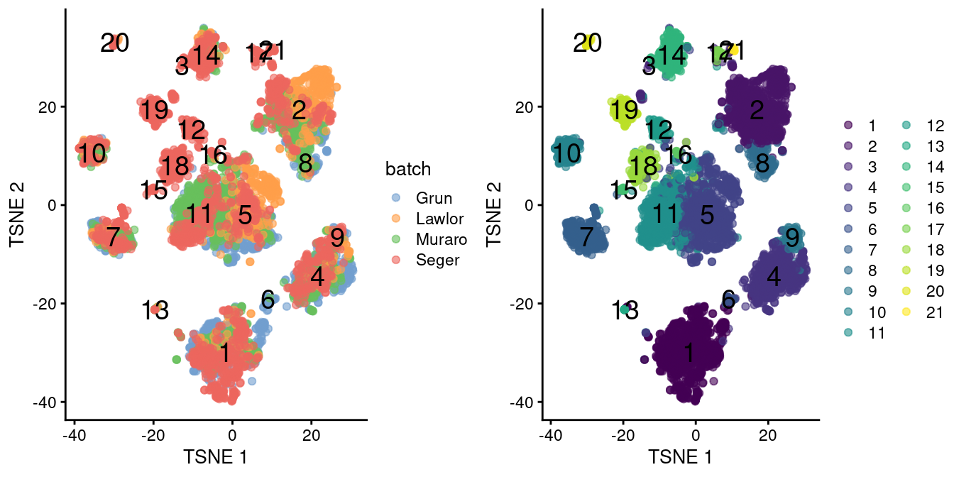
Figure 34.3: \(t\)-SNE plots of the four pancreas datasets after correction with fastMNN(). Each point represents a cell and is colored according to the batch of origin (left) or the assigned cluster (right). The cluster label is shown at the median location across all cells in the cluster.
Fortunately, we are battle-hardened and cynical, so we are sure to check for other sources of variation. The most obvious candidate is the donor of origin for each cell (Figure 34.4), which correlates strongly to these Segerstolpe-only clusters. This is not surprising given the large differences between humans in the wild, but donor-level variation is not interesting for the purposes of cell type characterization. (That said, preservation of the within-dataset donor effects is the technically correct course of action here, as a batch correction method should try to avoid removing heterogeneity within each of its defined batches.)
donors <- c(
    normed.pancreas$Grun$donor,
    normed.pancreas$Muraro$donor,
    normed.pancreas$Lawlor$`islet unos id`,
    normed.pancreas$Seger$Donor
)

seger.donors <- donors
seger.donors[mnn.pancreas$batch!="Seger"] <- NA
plotTSNE(mnn.pancreas, colour_by=I(seger.donors))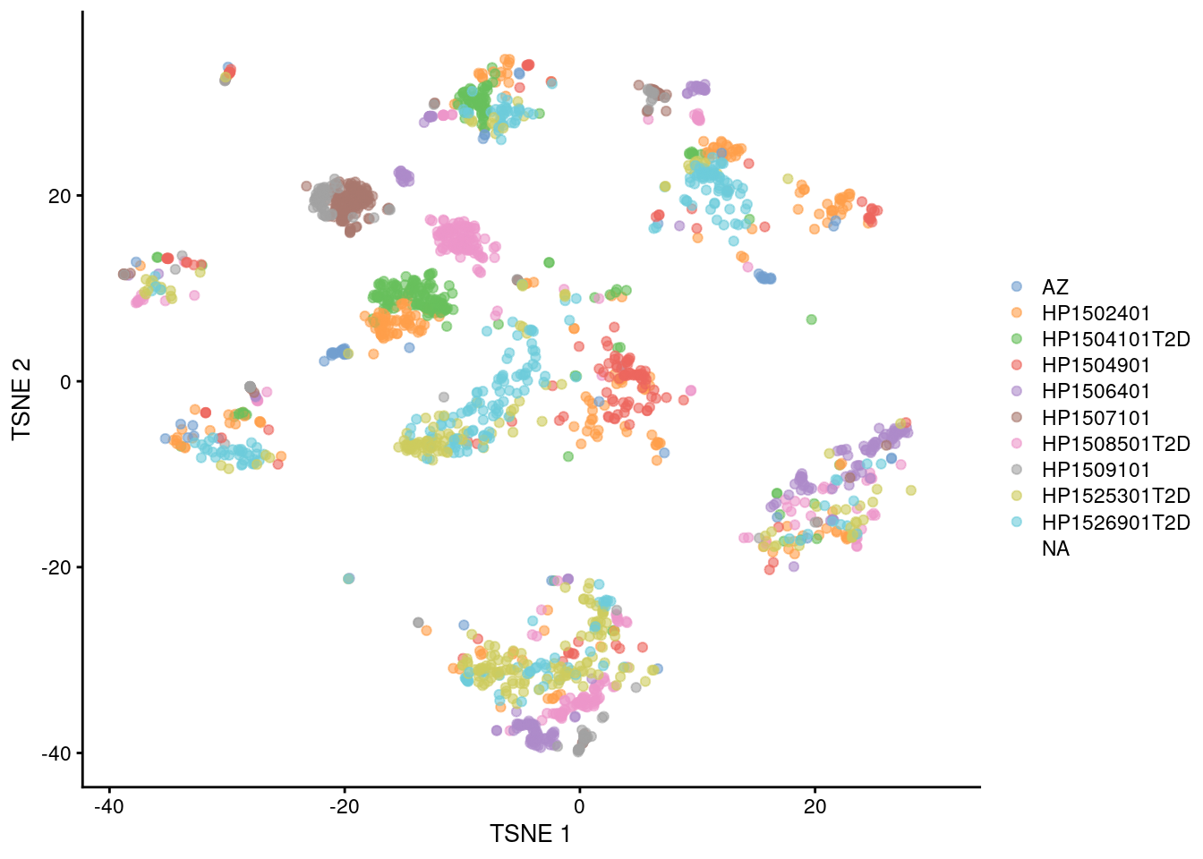
Figure 34.4: \(t\)-SNE plots of the four pancreas datasets after correction with fastMNN(). Each point represents a cell and is colored according to the donor of origin for the Segerstolpe dataset.
34.4 The ugly
Given these results, the most prudent course of action is to remove the donor effects within each dataset in addition to the batch effects across datasets.
This involves a bit more work to properly specify the two levels of unwanted heterogeneity.
To make our job a bit easier, we use the noCorrect() utility to combine all batches into a single SingleCellExperiment object.
We then call fastMNN() on the combined object with our chosen HVGs, using the batch= argument to specify which cells belong to which donors.
This will progressively merge cells from each donor in each batch until all cells are mapped onto a common coordinate space.
For some extra sophistication, we also set the weights= argument to ensure that each batch contributes equally to the PCA, regardless of the number of donors present in that batch; see ?multiBatchPCA for more details.
donors.per.batch <- split(combined$donor, combined$batch)
donors.per.batch <- lapply(donors.per.batch, unique)
donors.per.batch
## $Grun
## [1] "D2" "D3" "D7" "D10" "D17"
##
## $Lawlor
## [1] "ACIW009" "ACJV399" "ACCG268" "ACCR015A" "ACEK420A" "ACEL337" "ACHY057"
## [8] "ACIB065"
##
## $Muraro
## [1] "D28" "D29" "D31" "D30"
##
## $Seger
## [1] "HP1502401" "HP1504101T2D" "AZ" "HP1508501T2D" "HP1506401"
## [6] "HP1507101" "HP1509101" "HP1504901" "HP1525301T2D" "HP1526901T2D"set.seed(1010100)
multiout <- fastMNN(combined, batch=combined$donor,
subset.row=chosen.genes, weights=donors.per.batch)
# Renaming metadata fields for easier communication later.
multiout$dataset <- combined$batch
multiout$donor <- multiout$batch
multiout$batch <- NULLWith this approach, we see that the Segerstolpe-only clusters have disappeared (Figure 34.5). Visually, there also seems to be much greater mixing between cells from different Segerstolpe donors. This suggests that we have removed most of the donor effect, which simplifies the interpretation of our clusters.
library(scater)
g <- buildSNNGraph(multiout, use.dimred=1, k=20)
clusters <- igraph::cluster_walktrap(g)$membership
tab <- table(clusters, multiout$dataset)
tab
##
## clusters Grun Lawlor Muraro Seger
## 1 247 20 278 186
## 2 338 26 257 387
## 3 171 250 453 267
## 4 202 245 857 891
## 5 57 17 193 108
## 6 24 17 108 55
## 7 5 9 19 17
## 8 0 1 17 4
## 9 19 19 117 175multiout <- runTSNE(multiout, dimred="corrected")
gridExtra::grid.arrange(
plotTSNE(multiout, colour_by="dataset", text_by=I(clusters)),
plotTSNE(multiout, colour_by=I(seger.donors)),
ncol=2
)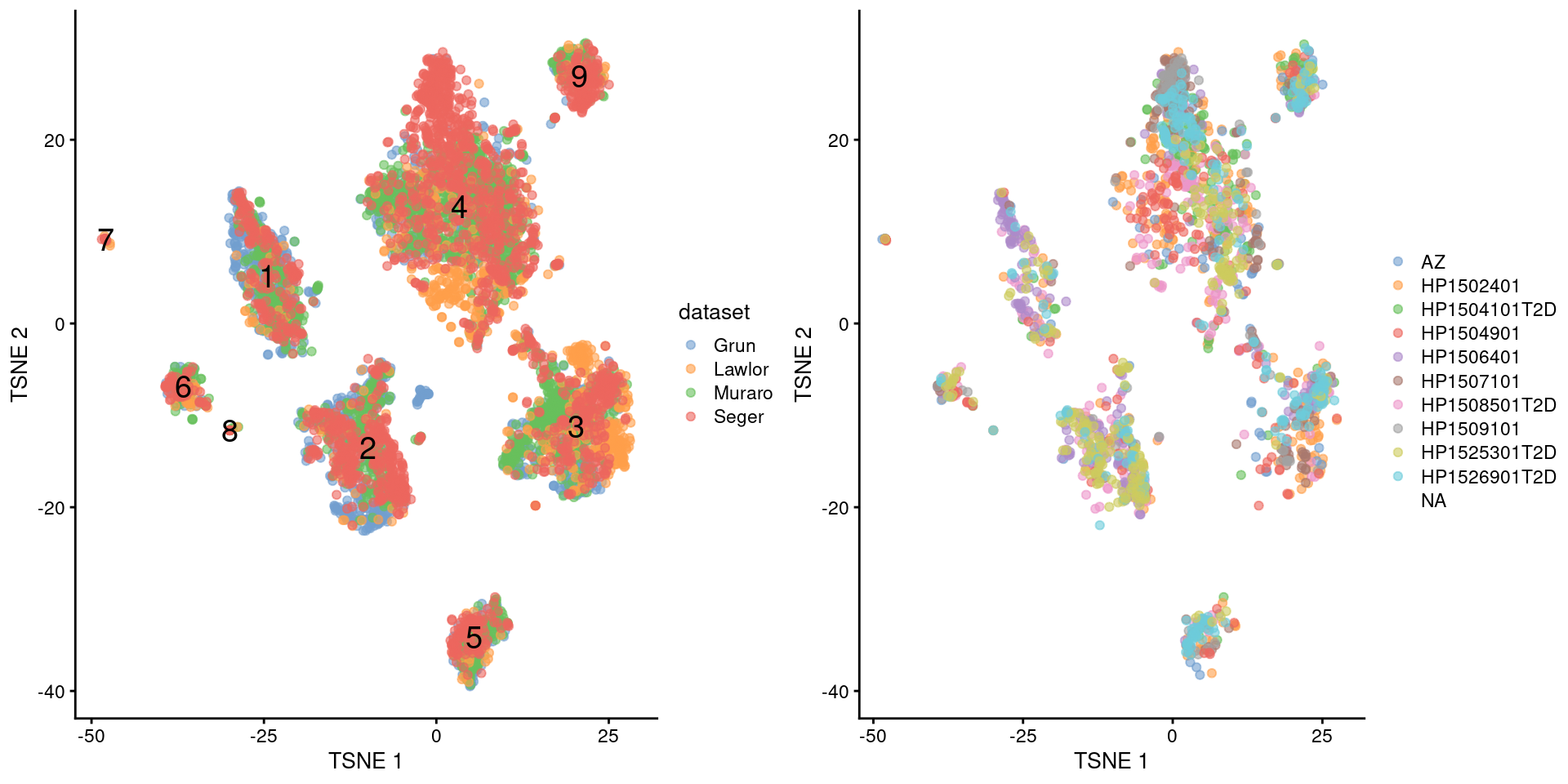
Figure 34.5: \(t\)-SNE plots of the four pancreas datasets after donor-level correction with fastMNN(). Each point represents a cell and is colored according to the batch of origin (left) or the donor of origin for the Segerstolpe-derived cells (right). The cluster label is shown at the median location across all cells in the cluster.
Our clusters compare well to the published annotations, indicating that we did not inadvertently discard important factors of variation during correction. (Though in this case, the cell types are so well defined, it would be quite a feat to fail to separate them!)
proposed <- c(rep(NA, ncol(sce.grun)),
    sce.muraro$label,
    sce.lawlor$`cell type`,
    sce.seger$CellType)

proposed <- tolower(proposed)
proposed[proposed=="gamma/pp"] <- "gamma"
proposed[proposed=="pp"] <- "gamma"
proposed[proposed=="duct"] <- "ductal"
proposed[proposed=="psc"] <- "stellate"
table(proposed, clusters)
## clusters
## proposed 1 2 3 4 5 6 7 8 9
## acinar 421 1 0 2 0 0 1 0 0
## alpha 1 7 4 1871 1 0 1 0 2
## beta 3 4 917 5 0 2 1 1 7
## co-expression 0 0 17 22 0 0 0 0 0
## delta 0 2 3 3 306 0 1 0 1
## ductal 6 612 4 1 0 6 0 10 1
## endothelial 0 0 0 0 0 1 33 0 0
## epsilon 0 0 0 2 0 0 0 0 6
## gamma 2 0 0 0 0 0 0 0 280
## mesenchymal 0 1 0 0 0 79 0 0 0
## mhc class ii 0 0 0 0 0 0 0 4 0
## nana 2 8 1 13 1 0 1 0 0
## none/other 0 3 1 2 0 0 4 1 1
## stellate 0 0 0 1 0 70 1 0 0
## unclassified 0 0 0 0 0 2 0 0 0
## unclassified endocrine 0 0 2 4 0 0 0 0 0
## unclear 0 4 0 0 0 0 0 0 0Session Info
R version 4.0.4 (2021-02-15)
Platform: x86_64-pc-linux-gnu (64-bit)
Running under: Ubuntu 20.04.2 LTS

Matrix products: default
BLAS:   /home/biocbuild/bbs-3.12-books/R/lib/libRblas.so
LAPACK: /home/biocbuild/bbs-3.12-books/R/lib/libRlapack.so

locale:
 [1] LC_CTYPE=en_US.UTF-8       LC_NUMERIC=C
 [3] LC_TIME=en_US.UTF-8        LC_COLLATE=C
 [5] LC_MONETARY=en_US.UTF-8    LC_MESSAGES=en_US.UTF-8
 [7] LC_PAPER=en_US.UTF-8       LC_NAME=C
 [9] LC_ADDRESS=C               LC_TELEPHONE=C
[11] LC_MEASUREMENT=en_US.UTF-8 LC_IDENTIFICATION=C

attached base packages:
[1] parallel  stats4    stats     graphics  grDevices utils     datasets
[8] methods   base

other attached packages:
 [1] bluster_1.0.0               scater_1.18.6
 [3] ggplot2_3.3.3               scran_1.18.5
 [5] batchelor_1.6.2             SingleCellExperiment_1.12.0
 [7] SummarizedExperiment_1.20.0 Biobase_2.50.0
 [9] GenomicRanges_1.42.0        GenomeInfoDb_1.26.4
[11] IRanges_2.24.1              S4Vectors_0.28.1
[13] BiocGenerics_0.36.0         MatrixGenerics_1.2.1
[15] matrixStats_0.58.0          BiocStyle_2.18.1
[17] rebook_1.0.0

loaded via a namespace (and not attached):
 [1] bitops_1.0-6              tools_4.0.4
 [3] bslib_0.2.4               utf8_1.2.1
 [5] R6_2.5.0                  irlba_2.3.3
 [7] ResidualMatrix_1.0.0      vipor_0.4.5
 [9] DBI_1.1.1                 colorspace_2.0-0
[11] withr_2.4.1               gridExtra_2.3
[13] tidyselect_1.1.0          processx_3.4.5
[15] compiler_4.0.4            graph_1.68.0
[17] BiocNeighbors_1.8.2       DelayedArray_0.16.2
[19] labeling_0.4.2            bookdown_0.21
[21] sass_0.3.1                scales_1.1.1
[23] callr_3.5.1               stringr_1.4.0
[25] digest_0.6.27             rmarkdown_2.7
[27] XVector_0.30.0            pkgconfig_2.0.3
[29] htmltools_0.5.1.1         sparseMatrixStats_1.2.1
[31] highr_0.8                 limma_3.46.0
[33] rlang_0.4.10              DelayedMatrixStats_1.12.3
[35] farver_2.1.0              jquerylib_0.1.3
[37] generics_0.1.0            jsonlite_1.7.2
[39] BiocParallel_1.24.1       dplyr_1.0.5
[41] RCurl_1.98-1.3            magrittr_2.0.1
[43] BiocSingular_1.6.0        GenomeInfoDbData_1.2.4
[45] scuttle_1.0.4             Matrix_1.3-2
[47] ggbeeswarm_0.6.0          Rcpp_1.0.6
[49] munsell_0.5.0             fansi_0.4.2
[51] viridis_0.5.1             lifecycle_1.0.0
[53] stringi_1.5.3             yaml_2.2.1
[55] edgeR_3.32.1              zlibbioc_1.36.0
[57] Rtsne_0.15                grid_4.0.4
[59] dqrng_0.2.1               crayon_1.4.1
[61] lattice_0.20-41           cowplot_1.1.1
[63] beachmat_2.6.4            locfit_1.5-9.4
[65] CodeDepends_0.6.5         knitr_1.31
[67] ps_1.6.0                  pillar_1.5.1
[69] igraph_1.2.6              codetools_0.2-18
[71] XML_3.99-0.6              glue_1.4.2
[73] evaluate_0.14             BiocManager_1.30.10
[75] vctrs_0.3.6               gtable_0.3.0
[77] purrr_0.3.4               assertthat_0.2.1
[79] xfun_0.22                 rsvd_1.0.3
[81] viridisLite_0.3.0         tibble_3.1.0
[83] beeswarm_0.3.1            statmod_1.4.35
[85] ellipsis_0.3.1
Bibliography
Grun, D., M. J. Muraro, J. C. Boisset, K. Wiebrands, A. Lyubimova, G. Dharmadhikari, M. van den Born, et al. 2016. “De Novo Prediction of Stem Cell Identity using Single-Cell Transcriptome Data.” Cell Stem Cell 19 (2): 266–77.
Lawlor, N., J. George, M. Bolisetty, R. Kursawe, L. Sun, V. Sivakamasundari, I. Kycia, P. Robson, and M. L. Stitzel. 2017. “Single-cell transcriptomes identify human islet cell signatures and reveal cell-type-specific expression changes in type 2 diabetes.” Genome Res. 27 (2): 208–22.
Muraro, M. J., G. Dharmadhikari, D. Grun, N. Groen, T. Dielen, E. Jansen, L. van Gurp, et al. 2016. “A Single-Cell Transcriptome Atlas of the Human Pancreas.” Cell Syst 3 (4): 385–94.
Segerstolpe, A., A. Palasantza, P. Eliasson, E. M. Andersson, A. C. Andreasson, X. Sun, S. Picelli, et al. 2016. “Single-Cell Transcriptome Profiling of Human Pancreatic Islets in Health and Type 2 Diabetes.” Cell Metab. 24 (4): 593–607.