Chapter 3 More counting options
3.1 Avoiding problematic genomic regions
Read extraction and counting can be restricted to particular chromosomes by specifying the names of the chromosomes of interest in restrict.
This avoids the need to count reads on unassigned contigs or uninteresting chromosomes, e.g., the mitochondrial genome for ChIP-seq studies targeting nuclear factors.
Alternatively, it allows windowCounts() to work on huge datasets or in limited memory by analyzing only one chromosome at a time.
Reads lying in certain regions can also be removed by specifying the coordinates of those regions in discard.
This is intended to remove reads that are wholly aligned within known repeat regions but were not removed by the minq filter.
Repeats are problematic as different repeat units in an actual genome are usually reported as a single unit in the genome build.
Alignment of all (non-specifically immunoprecipitated) reads from the former will result in artificially high coverage of the latter.
More importantly, any changes in repeat copy number or accessibility between conditions can lead to spurious DB at this single unit.
Removal of reads within repeat regions can avoid detection of these irrelevant differences.
repeats <- GRanges("chr1", IRanges(3000001, 3041000)) # telomere
discard.param <- readParam(discard=repeats)
Coordinates of annotated repeats can be obtained from several different sources.
- A curated blacklist of problematic regions is available from the ENCODE project (Consortium 2012) for various organisms. This list is constructed empirically from the ENCODE datasets and includes obvious offenders like telomeres, microsatellites and some rDNA genes. We generally prefer to use the ENCODE blacklist most applications where blacklisting is necessary.
- Alternatively, repeats can be predicted from the genome sequence using software like RepeatMasker.
These calls are available from the UCSC website (e.g., for mouse) or they can be extracted from an appropriate masked
BSgenomeobject. This contains a greater number of problematic regions (especially microsatellites) compared to the ENCODE blacklist, though genuine DB sites may also be removed. - If negative control samples are available, they can be used to empirically identify problematic regions with the GreyListChIP package. These regions should be ignored as they have high coverage in the controls and are unlikely to be genuine binding sites.
Using discard is more appropriate than simply ignoring windows that overlap the repeat regions.
For example, a large window might contain both repeat and non-repeat regions.
Discarding the window because of the former will compromise detection of DB features in the latter.
Of course, any DB sites within the discarded regions will be lost from downstream analyses.
Some caution is therefore required when specifying the regions of disinterest.
For example, many more repeats are called by RepeatMasker than are present in the ENCODE blacklist, so the use of the former may result in loss of potentially interesting features.
3.2 Increasing speed and memory efficiency
The spacing parameter controls the distance between adjacent windows in the genome.
By default, this is set to 50 bp, i.e., sliding windows are shifted 50 bp forward at each step.
Using a higher value will reduce computational work as fewer features need to be counted, and may be useful when machine memory is limited.
Of course, spatial resolution is lost with larger spacings as adjacent positions are not counted and thus cannot be distinguished.
#--- loading-files ---#
library(chipseqDBData)
tf.data <- NFYAData()
tf.data
bam.files <- head(tf.data$Path, -1) # skip the input.
bam.files

#--- counting-windows ---#
library(csaw)
frag.len <- 110
win.width <- 10
param <- readParam(minq=20)
data <- windowCounts(bam.files, ext=frag.len, width=win.width, param=param)
demo <- windowCounts(bam.files, spacing=100, ext=frag.len, width=win.width, param=param)
head(rowRanges(demo))## GRanges object with 6 ranges and 0 metadata columns:
## seqnames ranges strand
## <Rle> <IRanges> <Rle>
## [1] chr1 3003701-3003710 *
## [2] chr1 3003801-3003810 *
## [3] chr1 3004001-3004010 *
## [4] chr1 3008301-3008310 *
## [5] chr1 3008401-3008410 *
## [6] chr1 3010801-3010810 *
## -------
## seqinfo: 66 sequences from an unspecified genomeWhile the default is usually satisfactory, users can improve efficiency by increasing the spacing to a value up to (width + ext)/2.
This reduces the computational work by decreasing the number of windows and extracted counts.
Any loss in spatial resolution due to a larger spacing interval is negligible compared to that already lost by using a large window size.
The suggested upper bound ensures that a narrow binding site will not be overlooked if it falls between two windows.
Windows that are overlapped by few fragments are filtered out based on the filter argument.
A window is removed if the sum of counts across all libraries is below filter.
This improves memory efficiency by discarding the majority of low-abundance windows corresponding to uninteresting background regions.
The default value of the filter threshold is 10, though it can be raised to reduce memory usage for large libraries.
More sophisticated filtering is recommended and should be applied later (see Chapter~4).
demo <- windowCounts(bam.files, ext=frag.len, width=win.width,
    filter=30, param=param)
head(assay(demo))
## [,1] [,2] [,3] [,4]
## [1,] 4 12 10 5
## [2,] 5 6 8 11
## [3,] 7 1 9 19
## [4,] 3 1 7 22
## [5,] 4 2 10 15
## [6,] 6 5 10 11Users can parallelize read counting and several other functions by setting the BPPARAM argument.
This will load and process reads from multiple BAM files simultaneously.
The number of workers and type of parallelization can be specified using BiocParallelParam objects.
By default, parallelization is turned off (i.e., set to a SerialParam object) because it provides little benefit for small files or on systems with I/O bottlenecks.
3.3 Dealing with paired-end data
Paired-end datasets are accomodated by setting pe="both" in the param object supplied to windowCounts().
Read extension is not required as the genomic interval spanned by the originating fragment is explicitly defined as that between the 5’ positions of the paired reads.
The number of fragments overlapping each window is then counted as previously described.
By default, only proper pairs are used in which the two paired reads are on the same chromosome, face inward and are no more than max.frag apart.
# Using the BAM file in Rsamtools as an example.
pe.bam <- system.file("extdata", "ex1.bam", package="Rsamtools",
    mustWork=TRUE)

pe.param <- readParam(max.frag=400, pe="both")
demo <- windowCounts(pe.bam, ext=250, param=pe.param)
demo$totals
## [1] 1572A suitable value for max.frag is chosen by examining the distribution of fragment sizes from the getPESizes() function.
In this example, we might use a value of around 400 bp as it is larger than the vast majority of fragment sizes (Figure 3.1).
The plot can also be used to examine the quality of the PE sequencing procedure.
The location of the mode should be consistent with the fragmentation and size selection steps in library preparation.
out <- getPESizes(pe.bam)
frag.sizes <- out$sizes[out$sizes<=800]
hist(frag.sizes, breaks=50, xlab="Fragment sizes (bp)",
     ylab="Frequency", main="", col="grey80")
abline(v=400, col="red")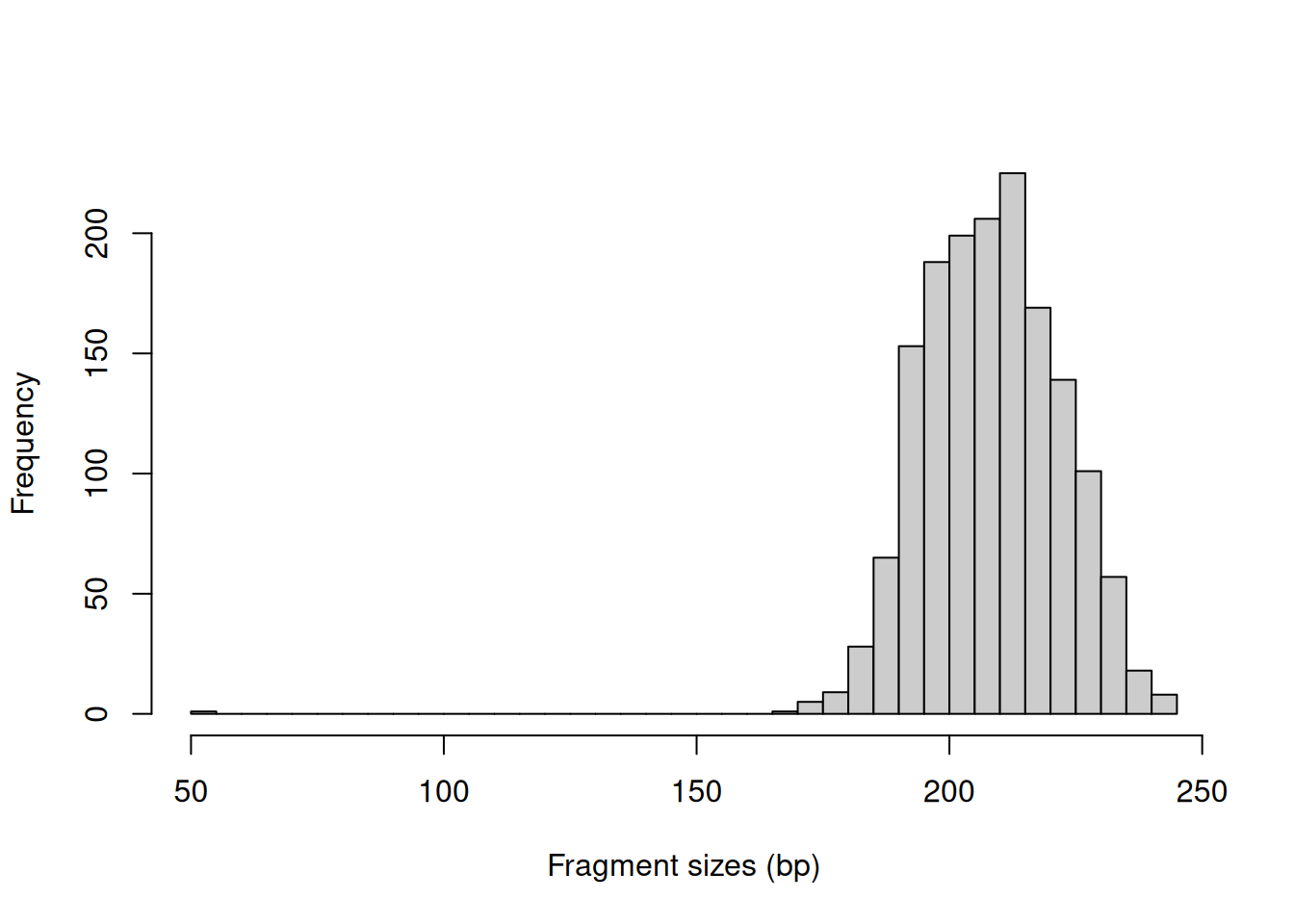
Figure 3.1: Distribution of fragment sizes in an example paired-end dataset.
The number of fragments exceeding the maximum size is recorded for quality control.
The getPESizes() function also returns the number of single reads, pairs with one unmapped read, improperly orientated pairs and inter-chromosomal pairs.
A non-negligble proportion of these reads may be indicative of problems with paired-end alignment or sequencing.
##   total.reads  mapped.reads        single mate.unmapped    unoriented
##          3307          3307             0           163             0
##     inter.chr     too.large
##             0             0
Note that all of the paired-end methods in csaw depend on correct mate information for each alignment. This is usually enforced by the aligner in the output BAM file. Any file manipulations that might break the synchronisation should be corrected (e.g., with the FixMateInformation program from the Picard suite) prior to read counting.
Paired-end data can also be treated as single-end by specifiying pe="first" or "second" in the readParam() constructor.
This will only use the first or second read of each read pair, regardless of the validity of the pair or the relative quality of the alignments.
This setting may be useful for contrasting paired- and single-end analyses, or in disastrous situations where paired-end sequencing has failed, e.g., due to ligation between DNA fragments.
## [1] 16543.4 Other counting strategies
3.4.1 Assigning reads into bins
Setting bin=TRUE will direct windowCounts() to count reads into contiguous bins across the genome.
Here, spacing is set to width such that each window forms a bin.
For single-end data, only the 5’ end of each read is used for counting into bins, without any directional extension.
For paired-end data, the midpoint of the originating fragment is used.)
## GRanges object with 6 ranges and 0 metadata columns:
##       seqnames          ranges strand
##          <Rle>       <IRanges>  <Rle>
##   [1]     chr1 3000001-3001000      *
##   [2]     chr1 3001001-3002000      *
##   [3]     chr1 3002001-3003000      *
##   [4]     chr1 3003001-3004000      *
##   [5]     chr1 3004001-3005000      *
##   [6]     chr1 3005001-3006000      *
##   -------
##   seqinfo: 66 sequences from an unspecified genome
The filter argument is automatically set to 1, which means that counts will be returned for each non-empty genomic bin.
Users should set width to a reasonably large value, to avoid running out of memory with a large number of small bins.
We can also force windowCounts() to return bins for all bins by setting filter=0 manually.
3.4.2 Manually specified regions
While csaw focuses on counting reads into windows,
it may be occasionally desirable to use the same conventions (e.g., duplicate removal, quality score filtering) when counting reads into pre-specified regions.
This can be performed with the regionCounts() function, which is largely a wrapper for countOverlaps() from the GenomicRanges package.
my.regions <- GRanges(c("chr11", "chr12", "chr15"),
    IRanges(c(75461351, 95943801, 21656501),
    c(75461610, 95944810, 21657610)))
reg.counts <- regionCounts(bam.files, my.regions, ext=frag.len, param=param)
head(assay(reg.counts))
## [,1] [,2] [,3] [,4]
## [1,] 43 68 116 111
## [2,] 1 0 0 0
## [3,] 17 10 14 123.4.3 Strand-specific counting
Techniques like CLIP-seq, MeDIP-seq or CAGE provide strand-specific sequence information.
csaw can analyze these datasets through strand-specific counting via the strandedCounts() wrapper function.
The strand of each output range indicates the strand on which reads were counted for that row.
Up to two rows can be generated for each window or region, depending on filtering.
ss.param <- initialize(param, forward=logical(0)) # flipping 'forward' to a new value.
ss.counts <- strandedCounts(bam.files, ext=frag.len, width=win.width, param=ss.param)
strand(rowRanges(ss.counts))
## factor-Rle of length 924432 with 72 runs
## Lengths: 67133 64898 22552 22019 38909 ... 1819 6 3 70 82
## Values : + - + - + ... - + - + -
## Levels(3): + - *Note that strandedCounts() operates internally by calling windowCounts() (or regionCounts()) twice with different settings for param$forward.
Specifically, setting forward=TRUE or FALSE would direct windowCounts() to only count reads on the forward or reverse strand.
strandedCounts() itself will only accept a logical(0) value for this slot, in order to protect the user;
any attempt to re-use ss.param in functions that are not designed for strand specificity will (appropriately) raise an error.
3.5 Handling variable fragment lengths
In rare cases, there will be large systematic differences in the fragment lengths between libraries.
For example, samples with less efficient fragmentation will exhibit larger fragment lengths and wider peaks.
Single-end reads in the peaks of such libraries will require more directional extension to impute a fragment interval that covers the binding site.
The windowCounts() function supports the use of library-specific fragment lengths, though some work is required to avoid detecting irrelevant DB from differences in peak widths.
This is achieved by resizing the inferred fragments to the same length in all libraries.
Consider a bimodal peak, present in several libraries that have different fragment lengths.
Resizing ensures that the subpeak on the forward strand is centered at the same location in each library - similarly, for the subpeak on the reverse strand.
Thus, the effect of differences in peak width between libraries can be largely mitigated.
Variable read extension is performed in windowCounts() by setting ext to a list with two elements.
The first element is a vector where each entry specifies the average fragment length to be used for the corresponding library.
The second specifies the final length to which the inferred fragments are to be resized.
If the second element is set to NA, no rescaling is performed and the library-specific fragment sizes are used directly.
This also works for analyses with paired-end data, though the first element of ext will be ignored as directional extension is not performed.
The example below rescales all fragments to 200 bp in all libraries.
Extension information is stored in the RangedSummarizedExperiment object for later use.
multi.frag.lens <- list(c(100, 150, 200, 250), 200)
demo <- windowCounts(bam.files, ext=multi.frag.lens, filter=30, param=param)
demo$ext
## [1] 100 150 200 250## [1] 200That said, use of different extension lengths is generally unnecessary in well-controlled datasets. Difference in lengths between libraries are usually smaller than 50 bp. This is less than the inherent variability in fragment lengths within each library (see the histogram for the paired-end data in Section~). The effect on the coverage profile of within-library variability in lengths will likely mask the effect of small between-library differences in the average lengths.
Session information
R version 4.6.0 RC (2026-04-17 r89917)
Platform: x86_64-pc-linux-gnu
Running under: Ubuntu 24.04.4 LTS

Matrix products: default
BLAS:   /home/biocbuild/bbs-3.23-bioc/R/lib/libRblas.so
LAPACK: /usr/lib/x86_64-linux-gnu/lapack/liblapack.so.3.12.0  LAPACK version 3.12.0

locale:
 [1] LC_CTYPE=en_US.UTF-8       LC_NUMERIC=C
 [3] LC_TIME=en_GB              LC_COLLATE=C
 [5] LC_MONETARY=en_US.UTF-8    LC_MESSAGES=en_US.UTF-8
 [7] LC_PAPER=en_US.UTF-8       LC_NAME=C
 [9] LC_ADDRESS=C               LC_TELEPHONE=C
[11] LC_MEASUREMENT=en_US.UTF-8 LC_IDENTIFICATION=C

time zone: America/New_York
tzcode source: system (glibc)

attached base packages:
[1] stats4    stats     graphics  grDevices utils     datasets  methods
[8] base

other attached packages:
 [1] csaw_1.46.0                 SummarizedExperiment_1.42.0
 [3] Biobase_2.72.0              MatrixGenerics_1.24.0
 [5] matrixStats_1.5.0           GenomicRanges_1.64.0
 [7] Seqinfo_1.2.0               IRanges_2.46.0
 [9] S4Vectors_0.50.0            BiocGenerics_0.58.0
[11] generics_0.1.4              BiocStyle_2.40.0
[13] rebook_1.22.0

loaded via a namespace (and not attached):
 [1] sass_0.4.10         SparseArray_1.12.0  bitops_1.0-9
 [4] lattice_0.22-9      digest_0.6.39       evaluate_1.0.5
 [7] grid_4.6.0          bookdown_0.46       fastmap_1.2.0
[10] jsonlite_2.0.0      Matrix_1.7-5        graph_1.90.0
[13] limma_3.68.0        BiocManager_1.30.27 Biostrings_2.80.0
[16] XML_3.99-0.23       codetools_0.2-20    jquerylib_0.1.4
[19] abind_1.4-8         cli_3.6.6           crayon_1.5.3
[22] CodeDepends_0.6.7   rlang_1.2.0         XVector_0.52.0
[25] cachem_1.1.0        DelayedArray_0.38.0 yaml_2.3.12
[28] metapod_1.20.0      otel_0.2.0          S4Arrays_1.12.0
[31] tools_4.6.0         dir.expiry_1.20.0   parallel_4.6.0
[34] BiocParallel_1.46.0 locfit_1.5-9.12     Rsamtools_2.28.0
[37] filelock_1.0.3      R6_2.6.1            lifecycle_1.0.5
[40] edgeR_4.10.0        bslib_0.10.0        Rcpp_1.1.1-1.1
[43] statmod_1.5.1       xfun_0.57           knitr_1.51
[46] htmltools_0.5.9     rmarkdown_2.31      compiler_4.6.0
Bibliography
Consortium, ENCODE Project. 2012. “An integrated encyclopedia of DNA elements in the human genome.” Nature 489 (7414): 57–74.