Chapter 4 Filtering out uninteresting windows
4.1 Overview
Many of the low abundance windows in the genome correspond to background regions in which DB is not expected. Indeed, windows with low counts will not provide enough evidence against the null hypothesis to obtain sufficiently low \(p\)-values for DB detection. Similarly, some approximations used in the statistical analysis will fail at low counts. Removing such uninteresting or ineffective tests reduces the severity of the multiple testing correction, increases detection power amongst the remaining tests and reduces computational work.
Filtering is valid so long as it is independent of the test statistic under the null hypothesis (Bourgon, Gentleman, and Huber 2010). In the negative binomial (NB) framework, this (probably) corresponds to filtering on the overall NB mean. The DB \(p\)-values retained after filtering on the overall mean should be uniform under the null hypothesis, by analogy to the normal case. Row sums can also be used for datasets where the effective library sizes are not very different, or where the counts are assumed to be Poisson-distributed between biological replicates.
In edgeR, the log-transformed overall NB mean is referred to as the average abundance.
This is computed with the aveLogCPM() function, as shown below for each window.
#--- loading-files ---#
library(chipseqDBData)
tf.data <- NFYAData()
tf.data
bam.files <- head(tf.data$Path, -1) # skip the input.
bam.files

#--- counting-windows ---#
library(csaw)
frag.len <- 110
win.width <- 10
param <- readParam(minq=20)
data <- windowCounts(bam.files, ext=frag.len, width=win.width, param=param)## Min. 1st Qu. Median Mean 3rd Qu. Max.
## -2.33 -2.30 -2.21 -2.14 -2.08 7.93For demonstration purposes, an arbitrary threshold of -1 is used here to filter the window abundances. This restricts the analysis to windows with abundances above this threshold.
##    Mode   FALSE    TRUE
## logical 4688607   15708
The exact choice of filter threshold may not be obvious. In particular, there is often no clear distinction in abundances between genuine binding and background events, e.g., due to the presence of many weak but genuine binding sites. A threshold that is too small will be ineffective, whereas a threshold that is too large may decrease power by removing true DB sites. Arbitrariness is unavoidable when balancing these opposing considerations.
Nonetheless, several strategies for defining the threshold are described below.
Users should start by choosing one of these filtering approaches to implement in their analyses.
Each approach yields a logical vector that can be used in the same way as keep.simple.
4.2 By count size
The simplest approach is to simply filter according to the count size. This removes windows for which the counts are simply too low for modelling and hypothesis testing. The code below retains windows with (library size-adjusted) average counts greater than 5.
##    Mode   FALSE    TRUE
## logical 4599548  104767
However, a count-based filter becomes less effective as the library size increases. More windows will be retained with greater sequencing depth, even in uninteresting background regions. This increases both computational work and the severity of the multiplicity correction. The threshold may also be inappropriate when library sizes are very different.
4.3 By proportion
One approach is to to assume that only a certain proportion - say, 0.1% - of the genome is genuinely bound.
This corresponds to the top proportion of high-abundance windows.
The total number of windows is calculated from the genome length and the spacing interval used in windowCounts().
The filterWindowsProportion() function returns the ratio of the rank of each window to this total, where higher-abundance windows have larger ranks.
Users can then retain those windows with rank ratios above the unbound proportion of the genome.
## [1] 54616This approach is simple and has the practical advantage of maintaining a constant number of windows for the downstream analysis. However, it may not adapt well to different datasets where the proportion of bound sites can vary. Using an inappropriate percentage of binding sites will result in the loss of potential DB regions or inclusion of background regions.
4.4 By global enrichment
An alternative approach involves choosing a filter threshold based on the fold change over the level of non-specific enrichment. The degree of background enrichment is estimated by counting reads into large bins across the genome. Binning is necessary here to increase the size of the counts when examining low-density background regions. This ensures that precision is maintained when estimating the background abundance.
The median of the average abundances across all bins is computed and used as a global estimate of the background coverage. This global background is then compared to the window-based abundances. This determines whether a window is driven by background enrichment, and thus, unlikely to be interesting. However, some care is required as the sizes of the regions used for read counting are different between bins and windows. The average abundance of each bin must be scaled down to be comparable to those of the windows.
The filterWindowsGlobal() function returns the increase in the abundance of each window over the global background.
Windows are filtered by setting some minimum threshold on this increase.
The aim is to eliminate the majority of uninteresting windows prior to further analysis.
Here, a fold change of 3 is necessary for a window to be considered as containing a binding site.
This approach has an intuitive and experimentally relevant interpretation that adapts to the level of non-specific enrichment in the dataset.
filter.stat <- filterWindowsGlobal(data, background=binned)
keep <- filter.stat$filter > log2(3)
sum(keep)
## [1] 23948We can visualize the effect of filtering (Figure 4.1) to confirm that the bulk of windows - presumably in background regions - are indeed discarded upon filtering. One might hope to see a bimodal distribution due to windows containing genuine binding sites, but this is usually not visible due to the dominance of background regions in the genome.
hist(filter.stat$filter, xlab="Log-fold change from global background",
    breaks=100, main="", col="grey80", xlim=c(0, 5))
abline(v=log2(3), col="red", lwd=2)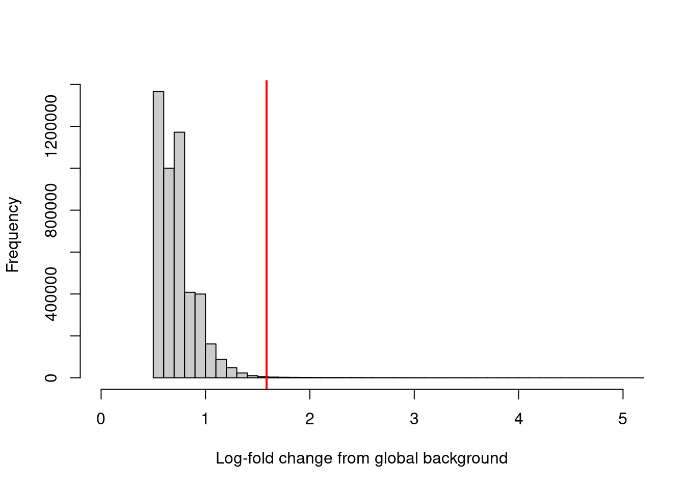
Figure 4.1: Distribution of the log-increase in coverage over the global background for each window in the NF-YA dataset. The red line denotes the chosen threshold for filtering.
Of course, the pre-specified minimum fold change may be too aggressive when binding is weak. For TF data, a large cut-off works well as narrow binding sites will have high read densities and are unlikely to be lost during filtering. Smaller minimum fold changes are recommended for diffuse marks where the difference from background is less obvious.
4.5 By local enrichment
4.5.1 Mimicking single-sample peak callers
Local background estimators can also be constructed, which avoids inappropriate filtering when there are differences in background coverage across the genome.
Here, the 2 kbp region surrounding each window will be used as the “neighborhood” over which a local estimate of non-specific enrichment for that window can be obtained.
The counts for these regions are first obtained with the regionCounts() function.
This should be synchronized with windowCounts() by using the same param, if any non-default settings were used.
surrounds <- 2000
neighbor <- suppressWarnings(resize(rowRanges(data), surrounds, fix="center"))
wider <- regionCounts(bam.files, regions=neighbor, ext=frag.len, param=param)
We apply filterWindowsLocal() to compute enrichment values, i.e., the increase in the abundance of each window over its neighborhood.
In this function, counts for each window are subtracted from the counts for its neighborhood.
This ensures that any enriched regions or binding sites inside the window will not interfere with estimation of its local background.
The width of the window is also subtracted from that of its neighborhood, to reflect the effective size of the latter after subtraction of counts.
Based on the fold-differences in widths, the abundance of the neighborhood is scaled down for a valid comparison to that of the corresponding window.
Enrichment values are subsequently calculated from the differences in scaled abundances.
##    Min. 1st Qu.  Median    Mean 3rd Qu.    Max.
##  -6.287   0.438   0.575   0.588   0.727   8.149
Filtering can then be performed using a quantile- or fold change-based threshold on the enrichment values. In this scenario, a 3-fold increase in enrichment over the neighborhood abundance is required for retention of each window (Figure 4.2). This roughly mimics the behavior of single-sample peak-calling programs such as MACS (Zhang et al. 2008).
## [1] 10701hist(filter.stat$filter, xlab="Log-fold change from local background",
breaks=100, main="", col="grey80", xlim=c(0, 5))
abline(v=log2(3), col="red", lwd=2)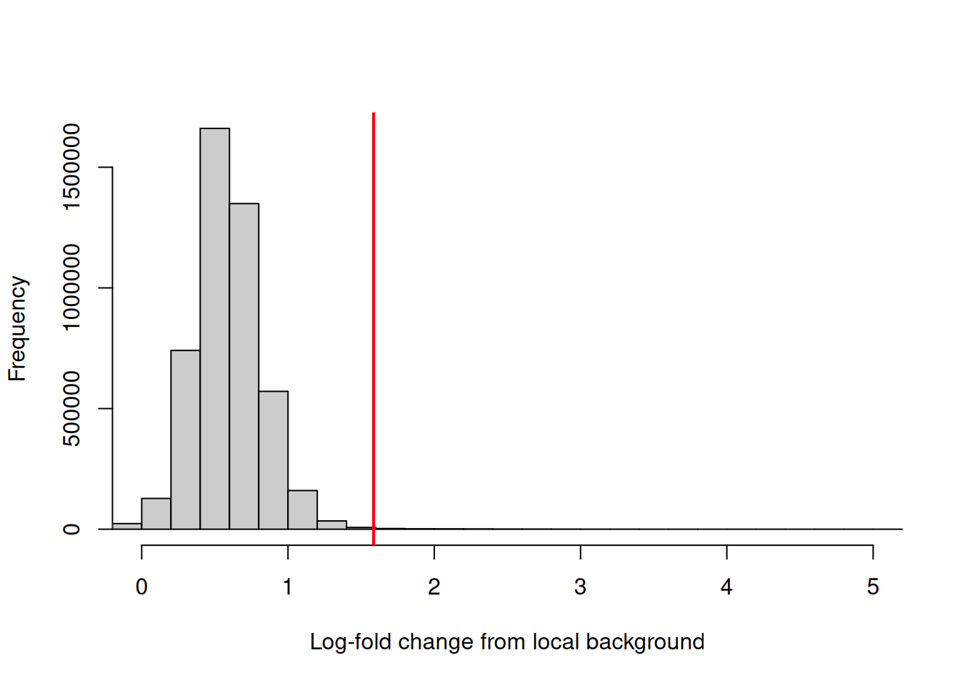
Figure 4.2: Distribution of the log-increase in coverage over the local background for each window in the NF-YA dataset. The red line denotes the chosen threshold for filtering.
Note that this procedure also assumes that no other enriched regions are present in each neighborhood. Otherwise, the local background will be overestimated and windows may be incorrectly filtered out. This may be problematic for diffuse histone marks or clusters of TF binding sites, where enrichment may be observed in both the window and its neighborhood.
If this seems too complicated, an alternative is to identify locally enriched regions using peak-callers like MACS.
Filtering can then be performed to retain only windows within called peaks.
However, peak calling must be done independently of the DB status of each window.
If libraries are of similar size or biological variability is low, reads can be pooled into one library for single-sample peak calling (Lun and Smyth 2014).
This is equivalent to filtering on the average count and avoids loss of the type I error control from data snooping.
4.5.2 Identifying local maxima {sec:localmax}
Another strategy is to use the findMaxima() function to identify local maxima in the read density across the genome.
The code below will determine if each window is a local maximum, i.e., whether it has the highest average abundance within 1 kbp on either side.
The data can then be filtered to retain only these locally maximal windows.
This can also be combined with other filters to ensure that the retained windows have high absolute abundance.
##    Mode   FALSE    TRUE
## logical 3782693  921622
This approach is very aggressive and should only be used (sparingly) in datasets where binding is sharp, simple and isolated. Complex binding events involving diffuse enrichment or adjacent binding sites will not be handled well. For example, DB detection will fail if a low-abundance DB window is ignored in favor of a high-abundance non-DB neighbor.
4.6 With negative controls
Negative controls for ChIP-seq refer to input or IgG libraries where the IP step has been skipped or compromised with an irrelevant antibody, respectively. This accounts for sequencing/mapping biases in ChIP-seq data. IgG controls also quantify the amount of non-specific enrichment throughout the genome. These controls are mostly irrelevant when testing for DB between ChIP samples. However, they can be used to filter out windows where the average abundance across the ChIP samples is below the abundance of the control. To illustrate, let us add an input library to our NF-YA data set in the code below.
library(chipseqDBData)
tf.data <- NFYAData()
with.input <- tf.data$Path
in.demo <- windowCounts(with.input, ext=frag.len, param=param)
chip <- in.demo[,1:4] # All ChIP libraries
control <- in.demo[,5] # All control libraries
Some additional work is required to account for composition biases that are likely to be present when comparing ChIP to negative control samples (see Section 5.2).
A simple strategy for normalization involves counting reads into large bins, which are used in scaleControlFilter() to compute a normalization factor.
in.binned <- windowCounts(with.input, bin=TRUE, width=10000, param=param)
chip.binned <- in.binned[,1:4]
control.binned <- in.binned[,5]
scale.info <- scaleControlFilter(chip.binned, control.binned)
We use the filterWindowsControl() function to compute the enrichment of the ChIP counts over the control counts for each window.
This uses scale.info to adjust for composition biases between ChIP and control samples.
A larger prior.count of 5 is also used to compute the average abundance.
This protects against inflated log-fold changes when the count for the window in the control sample is near zero.1
The log-fold enrichment of the ChIP sample over the control is then computed for each window, after normalizing for composition bias with the binned counts. The example below requires a 3-fold or greater increase in abundance over the control to retain each window (Figure 4.3).
## [1] 6657hist(filter.stat$filter, xlab="Log-fold change from control",
breaks=100, main="", col="grey80", xlim=c(0, 5))
abline(v=log2(3), col="red", lwd=2)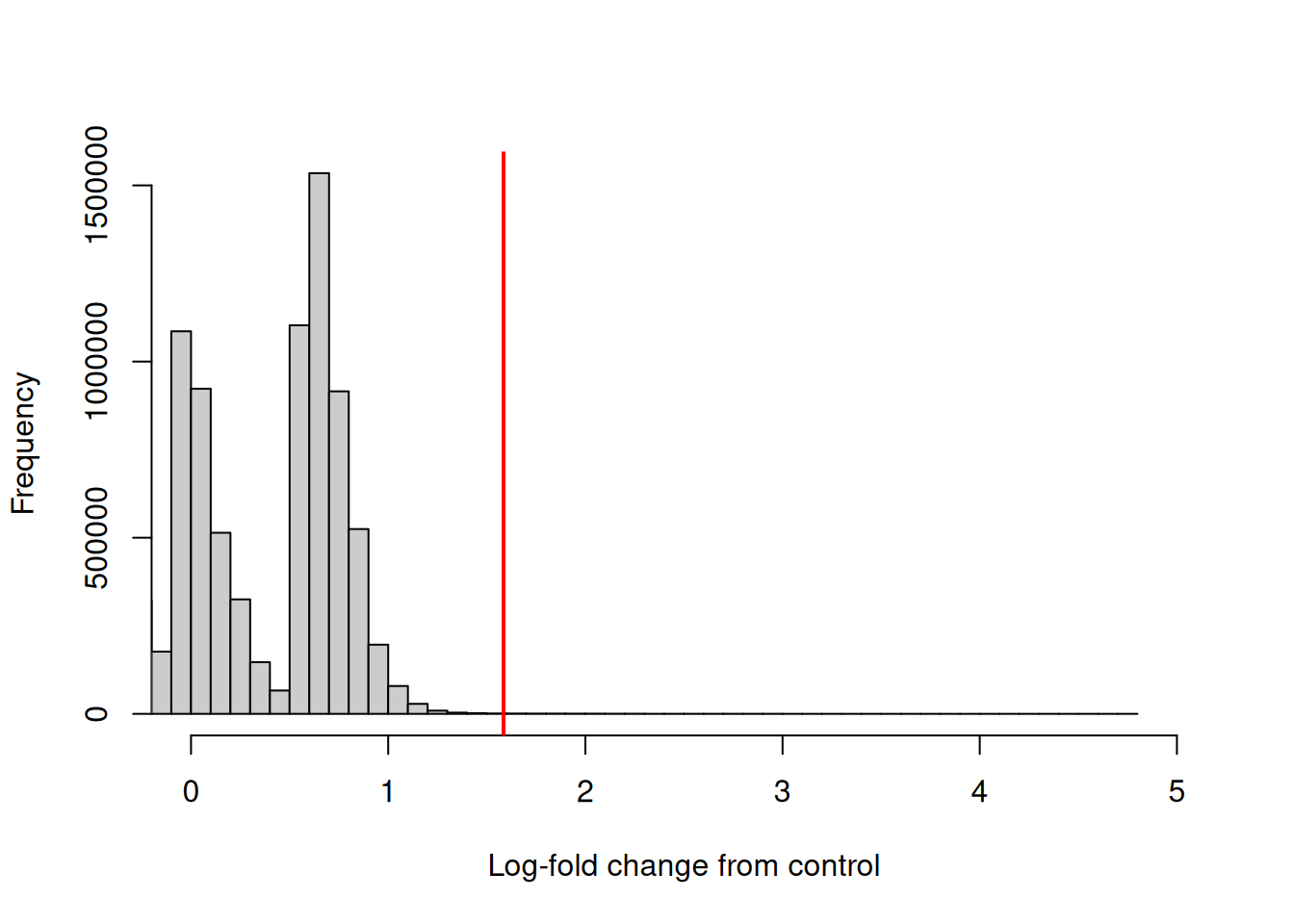
Figure 4.3: Distribution of the log-increase in average abundance for the ChIP samples over the control for each window in the NF-YA dataset. The red line denotes the chosen threshold for filtering.
As an aside, the csaw pipeline can also be applied to search for DB'' between ChIP libraries and control libraries. The ChIP and control libraries can be treated as separate groups, in which mostDB’’ events are expected to be enriched in the ChIP samples.
If this is the case, the filtering procedure described above is inappropriate as it will select for windows with differences between ChIP and control samples.
This compromises the assumption of the null hypothesis during testing, resulting in loss of type I error control.
4.7 By prior information
When only a subset of genomic regions are of interest, DB detection power can be improved by removing windows lying outside of these regions. Such regions could include promoters, enhancers, gene bodies or exons. Alternatively, sites could be defined from a previous experiment or based on the genome sequence, e.g., TF motif matches. The example below retrieves the coordinates of the broad gene bodies from the mouse genome, including the 3 kbp region upstream of the TSS that represents the putative promoter region for each gene.
library(TxDb.Mmusculus.UCSC.mm10.knownGene)
broads <- genes(TxDb.Mmusculus.UCSC.mm10.knownGene)
broads <- resize(broads, width(broads)+3000, fix="end")
head(broads)
## GRanges object with 6 ranges and 1 metadata column:
## seqnames ranges strand | gene_id
## <Rle> <IRanges> <Rle> | <character>
## 100009600 chr9 21062393-21076096 - | 100009600
## 100009609 chr7 84935565-84967115 - | 100009609
## 100009614 chr10 77708457-77712009 + | 100009614
## 100009664 chr11 45805087-45841171 + | 100009664
## 100012 chr4 144157557-144165663 - | 100012
## 100017 chr4 134741554-134771024 - | 100017
## -------
## seqinfo: 66 sequences (1 circular) from mm10 genomeWindows can be filtered to only retain those which overlap with the regions of interest. Discerning users may wish to distinguish between full and partial overlaps, though this should not be a significant issue for small windows. This could also be combined with abundance filtering to retain windows that contain putative binding sites in the regions of interest.
## [1] 2700568Any information used here should be independent of the DB status under the null in the current dataset. For example, DB calls from a separate dataset and/or independent annotation can be used without problems. However, using DB calls from the same dataset to filter regions would violate the null assumption and compromise type I error control.
In addition, this filter is unlike the others in that it does not operate on the abundance of the windows. It is possible that the set of retained windows may be very small, e.g., if no non-empty windows overlap the pre-defined regions of interest. Thus, it may be better to apply this filter before the multiplicity correction but after DB testing. This ensures that there are sufficient windows for stable estimation of the downstream statistics.
4.8 Some final comments about filtering
It should be stressed that these filtering strategies do not eliminate subjectivity. Some thought is still required in selecting an appropriate proportion of bound sites or minimum fold change above background for each method. Rather, these filters provide a relevant interpretation for what would otherwise be an arbitrary threshold on the abundance.
As a general rule, users should filter less aggressively if there is any uncertainty about the features of interest. In particular, the thresholds shown in this chapter for each filtering statistic are fairly mild. This ensures that more potentially DB windows are retained for testing. Use of an aggressive filter risks the complete loss of detection for such windows, even if power is improved among those that are retained. Low numbers of retained windows may also lead to unstable estimates during, e.g., normalization, variance modelling.
Different filters can also be combined in more advanced applications, e.g., by running for filter vectors {keep1} and \Robject{keep2().
Any benefit will depend on the type of filters involved.
The greatest effect is observed for filters that operate on different principles.
For example, the low-count filter can be combined with others to ensure that all retained windows surpass some minimum count.
This is especially relevant for the local background filters, where a large enrichment value does not guarantee a large count.
Session information
R version 4.6.0 RC (2026-04-17 r89917)
Platform: x86_64-pc-linux-gnu
Running under: Ubuntu 24.04.4 LTS

Matrix products: default
BLAS:   /home/biocbuild/bbs-3.23-bioc/R/lib/libRblas.so
LAPACK: /usr/lib/x86_64-linux-gnu/lapack/liblapack.so.3.12.0  LAPACK version 3.12.0

locale:
 [1] LC_CTYPE=en_US.UTF-8       LC_NUMERIC=C
 [3] LC_TIME=en_GB              LC_COLLATE=C
 [5] LC_MONETARY=en_US.UTF-8    LC_MESSAGES=en_US.UTF-8
 [7] LC_PAPER=en_US.UTF-8       LC_NAME=C
 [9] LC_ADDRESS=C               LC_TELEPHONE=C
[11] LC_MEASUREMENT=en_US.UTF-8 LC_IDENTIFICATION=C

time zone: America/New_York
tzcode source: system (glibc)

attached base packages:
[1] stats4    stats     graphics  grDevices utils     datasets  methods
[8] base

other attached packages:
 [1] TxDb.Mmusculus.UCSC.mm10.knownGene_3.10.0
 [2] GenomicFeatures_1.64.0
 [3] AnnotationDbi_1.74.0
 [4] chipseqDBData_1.27.0
 [5] edgeR_4.10.0
 [6] limma_3.68.0
 [7] csaw_1.46.0
 [8] SummarizedExperiment_1.42.0
 [9] Biobase_2.72.0
[10] MatrixGenerics_1.24.0
[11] matrixStats_1.5.0
[12] GenomicRanges_1.64.0
[13] Seqinfo_1.2.0
[14] IRanges_2.46.0
[15] S4Vectors_0.50.0
[16] BiocGenerics_0.58.0
[17] generics_0.1.4
[18] BiocStyle_2.40.0
[19] rebook_1.22.0

loaded via a namespace (and not attached):
 [1] tidyselect_1.2.1         dplyr_1.2.1              blob_1.3.0
 [4] filelock_1.0.3           Biostrings_2.80.0        bitops_1.0-9
 [7] RCurl_1.98-1.18          fastmap_1.2.0            BiocFileCache_3.2.0
[10] GenomicAlignments_1.48.0 XML_3.99-0.23            digest_0.6.39
[13] lifecycle_1.0.5          statmod_1.5.1            KEGGREST_1.52.0
[16] RSQLite_2.4.6            magrittr_2.0.5           compiler_4.6.0
[19] rlang_1.2.0              sass_0.4.10              tools_4.6.0
[22] yaml_2.3.12              rtracklayer_1.72.0       knitr_1.51
[25] S4Arrays_1.12.0          bit_4.6.0                curl_7.1.0
[28] DelayedArray_0.38.0      abind_1.4-8              BiocParallel_1.46.0
[31] withr_3.0.2              purrr_1.2.2              CodeDepends_0.6.7
[34] grid_4.6.0               ExperimentHub_3.2.0      cli_3.6.6
[37] rmarkdown_2.31           crayon_1.5.3             otel_0.2.0
[40] metapod_1.20.0           rjson_0.2.23             httr_1.4.8
[43] DBI_1.3.0                cachem_1.1.0             parallel_4.6.0
[46] restfulr_0.0.16          BiocManager_1.30.27      XVector_0.52.0
[49] vctrs_0.7.3              Matrix_1.7-5             jsonlite_2.0.0
[52] dir.expiry_1.20.0        bookdown_0.46            bit64_4.8.0
[55] locfit_1.5-9.12          jquerylib_0.1.4          glue_1.8.1
[58] codetools_0.2-20         BiocVersion_3.23.1       BiocIO_1.22.0
[61] tibble_3.3.1             pillar_1.11.1            rappdirs_0.3.4
[64] htmltools_0.5.9          graph_1.90.0             R6_2.6.1
[67] dbplyr_2.5.2             httr2_1.2.2              evaluate_1.0.5
[70] lattice_0.22-9           AnnotationHub_4.2.0      cigarillo_1.2.0
[73] png_0.1-9                Rsamtools_2.28.0         memoise_2.0.1
[76] bslib_0.10.0             Rcpp_1.1.1-1.1           SparseArray_1.12.0
[79] xfun_0.57                pkgconfig_2.0.3
Bibliography
Bourgon, R., R. Gentleman, and W. Huber. 2010. “Independent filtering increases detection power for high-throughput experiments.” Proc. Natl. Acad. Sci. U.S.A. 107 (21): 9546–51.
Lun, A. T., and G. K. Smyth. 2014. “De novo detection of differentially bound regions for ChIP-seq data using peaks and windows: controlling error rates correctly.” Nucleic Acids Res. 42 (11): e95.
Zhang, Y., T. Liu, C. A. Meyer, J. Eeckhoute, D. S. Johnson, B. E. Bernstein, C. Nusbaum, et al. 2008. “Model-based analysis of ChIP-Seq (MACS).” Genome Biol. 9 (9): R137.
By comparison, the global and local background estimates require less protection (
prior.count=2, by default) as they are derived from larger bins with more counts.↩︎