Chapter 6 Testing for per-window differences
6.1 Overview
Low counts per window are typically observed in ChIP-seq datasets, even for genuine binding sites. Any statistical analysis to identify DB sites must be able to handle discreteness in the data. Count-based models are ideal for this purpose. In this guide, the quasi-likelihood (QL) framework in the edgeR package is used (Lund et al. 2012). Counts are modelled using NB distributions that account for overdispersion between biological replicates (Robinson and Smyth 2008). Each window can then be tested for significant DB between conditions.
Of course, any statistical method can be used if it is able to accept a count matrix and a vector of normalization factors (or more generally, a matrix of offsets). The choice of edgeR is primarily motivated by its performance relative to some published alternatives (Law et al. 2014)2.
6.2 Setting up for edgeR
A DGEList object is first constructed from the SummarizedExperiment contaiing our filtered count matrix.
If normalization factors or offsets are present in the RangedSummarizedExperiment object – see Chapter~5 – they will automatically be inserted into the DGEList.
Otherwise, they can be manually passed to the asDGEList() function.
If offsets are available, they will generally override the normalization factors in the downstream edgeR analysis.
#--- loading-files ---#
library(chipseqDBData)
tf.data <- NFYAData()
tf.data
bam.files <- head(tf.data$Path, -1) # skip the input.
bam.files

#--- counting-windows ---#
library(csaw)
frag.len <- 110
win.width <- 10
param <- readParam(minq=20)
data <- windowCounts(bam.files, ext=frag.len, width=win.width, param=param)

#--- filtering ---#
binned <- windowCounts(bam.files, bin=10000, param=param)
fstats <- filterWindowsGlobal(data, binned)
filtered.data <- data[fstats$filter > log2(5),]

#--- normalization ---#
filtered.data <- normFactors(binned, se.out=filtered.data)The experimental design is described by a design matrix.
In this case, the only relevant factor is the cell type of each sample.
A generalized linear model (GLM) will be fitted to the counts for each window using the specified design (McCarthy, Chen, and Smyth 2012).
This provides a general framework for the analysis of complex experiments with multiple factors.
In this case, our design matrix contains an intercept representing the average abundance in the ESC group,
plus a cell.type coefficient representing the log-fold change of the TN group over the ESC group.
## [1] "ESC" "ESC" "TN" "TN"## intercept cell.type
## 1 1 0
## 2 1 0
## 3 1 1
## 4 1 1
## attr(,"assign")
## [1] 0 1
## attr(,"contrasts")
## attr(,"contrasts")$`factor(cell.type)`
## [1] "contr.treatment"Readers are referred to the user’s guide in edgeR for more details on parametrization of the design matrix.
6.3 Estimating the dispersions
6.3.1 Stabilising estimates with empirical Bayes
Under the QL framework, both the QL and NB dispersions are used to model biological variability in the data (Lund et al. 2012). The former ensures that the NB mean-variance relationship is properly specified with appropriate contributions from the Poisson and Gamma components. The latter accounts for variability and uncertainty in the dispersion estimate. However, limited replication in most ChIP-seq experiments means that each window does not contain enough information for precise estimation of either dispersion.
This problem is overcome in edgeR by sharing information across windows.
For the NB dispersions, a mean-dispersion trend is fitted across all windows to model the mean-variance relationship (McCarthy, Chen, and Smyth 2012).
The raw QL dispersion for each window is estimated after fitting a GLM with the trended NB dispersion.
Another mean-dependent trend is fitted to the raw QL estimates.
An empirical Bayes (EB) strategy is then used to stabilize the raw QL dispersion estimates by shrinking them towards the second trend (Lund et al. 2012).
The ideal amount of shrinkage is determined from the variability of the dispersions.
##    Min. 1st Qu.  Median    Mean 3rd Qu.    Max.
## 0.0592 0.1017 0.1047 0.1043 0.1076 0.1087## Length Class Mode
## 0 NULL NULLThe effect of EB stabilisation can be visualized by examining the biological coefficient of variation (for the NB dispersion) and the quarter-root deviance (for the QL dispersion). Plot such as those in Figure 6.1 can also be used to decide whether the fitted trend is appropriate. Sudden irregulaties may be indicative of an underlying structure in the data which cannot be modelled with the mean-dispersion trend. Discrete patterns in the raw dispersions are indicative of low counts and suggest that more aggressive filtering is required.
par(mfrow=c(1,2))
o <- order(y$AveLogCPM)
plot(y$AveLogCPM[o], sqrt(y$trended.dispersion[o]), type="l", lwd=2,
     ylim=c(0, 1), xlab=expression("Ave."~Log[2]~"CPM"),
     ylab=("Biological coefficient of variation"))
plotQLDisp(fit)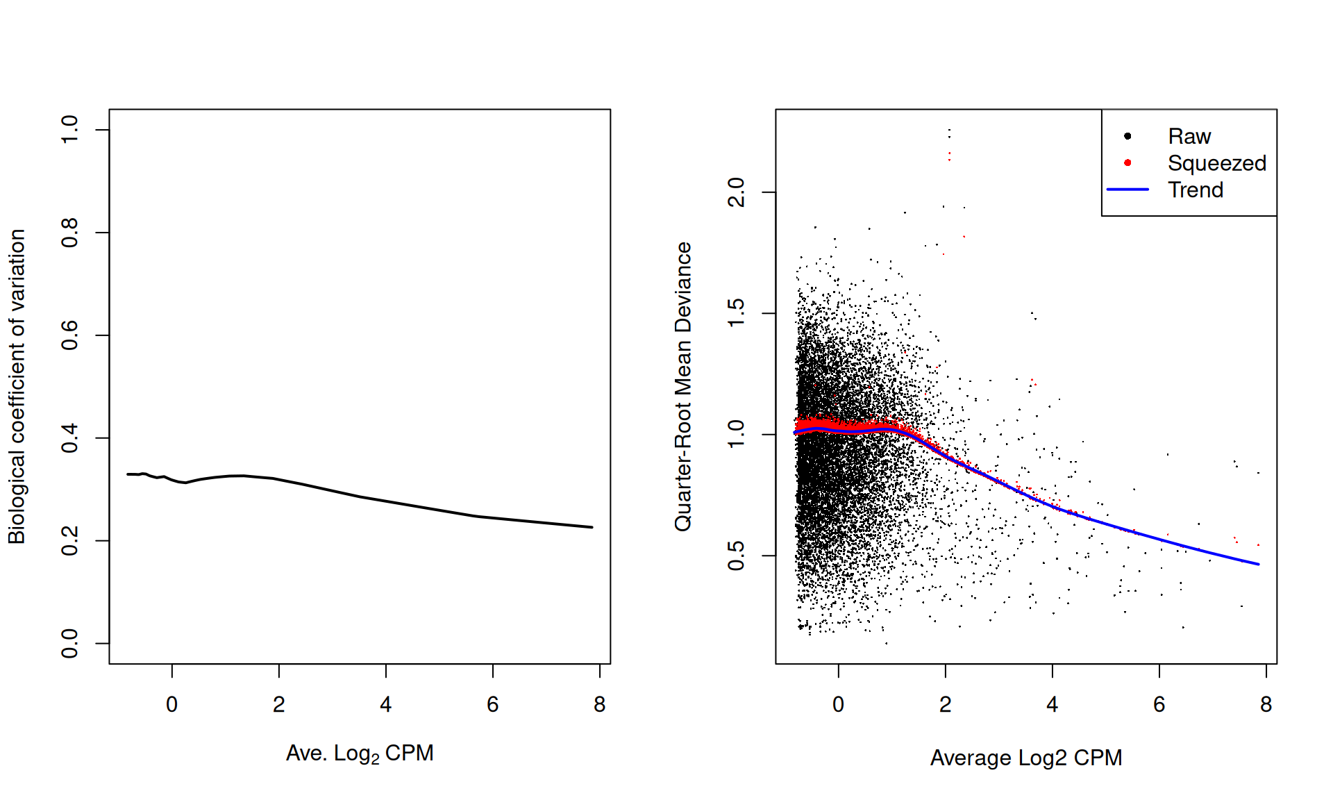
Figure 6.1: Fitted trend in the NB dispersion (left) or QL dispersion (right) as a function of the average abundance for each window. For the NB dispersion, the square root is shown as the biological coefficient of variation. For the QL dispersion, the shrunken estimate is also shown for each window.
For most sequencing count data, we expect to see a decreasing trend that plateaus with increasing average abundance. This reflects the greater reliability of large counts, where the effects of stochasticity and technical artifacts (e.g., mapping errors, PCR duplicates) are averaged out. In some cases, a strong trend may also be observed where the NB dispersion drops sharply with increasing average abundance. It is difficult to accurately fit an empirical curve to these strong trends, and as a consequence, the dispersions at high abundances may be overestimated. Filtering of low-abundance regions (as described in Chapter 4) provides some protection by removing the strongest part of the trend. This has an additional benefit of removing those tests that have low power due to the magnitude of the dispersions.
relevant <- rowSums(assay(data)) >= 20 # weaker filtering than 'filtered.data'
yo <- asDGEList(data[relevant,], norm.factors=filtered.data$norm.factors)
yo <- estimateDisp(yo, design)
oo <- order(yo$AveLogCPM)

plot(yo$AveLogCPM[oo], sqrt(yo$trended.dispersion[oo]), type="l", lwd=2,
     ylim=c(0, max(sqrt(yo$trended))), xlab=expression("Ave."~Log[2]~"CPM"),
     ylab=("Biological coefficient of variation"))
lines(y$AveLogCPM[o], sqrt(y$trended[o]), lwd=2, col="grey")
legend("topright", c("raw", "filtered"), col=c("black", "grey"), lwd=2)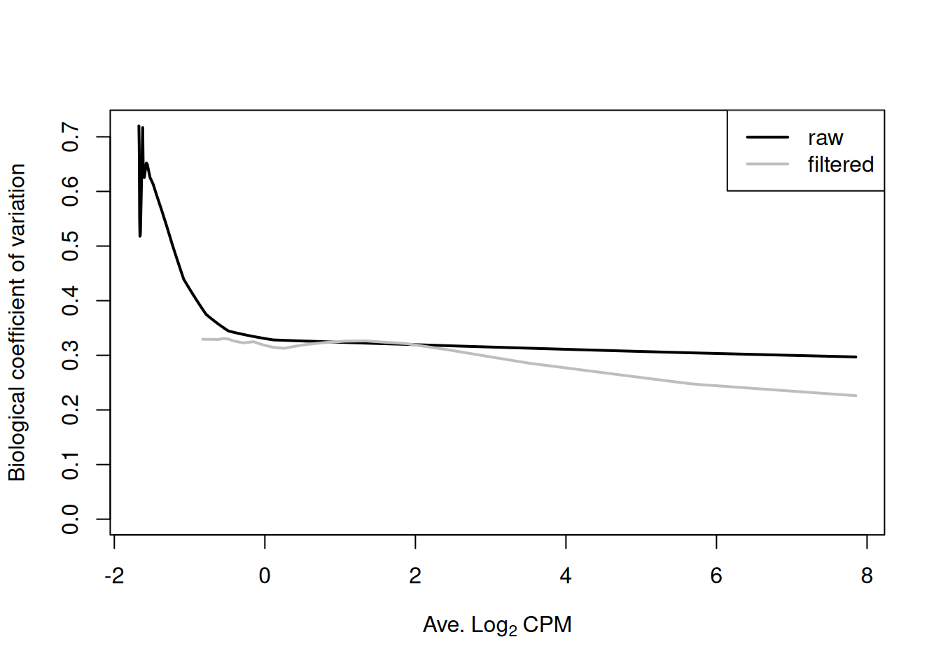
Figure 6.2: Fitted trend in the NB dispersions before (black) and after (grey) removing low-abundance windows.
Note that only the trended dispersion will be used in the downstream steps – the common and tagwise values are only shown in Figure 6.1 for diagnostic purposes. Specifically, the common BCV provides an overall measure of the variability in the data set, averaged across all windows. The tagwise BCVs should also be dispersed above and below the fitted trend, indicating that the fit was successful.
6.3.2 Modelling variable dispersions between windows
Any variability in the dispersions across windows is modelled in edgeR by the prior degrees of freedom (d.f.). A large value for the prior d.f. indicates that the variability is low. This means that more EB shrinkage can be performed to reduce uncertainty and maximize power. However, strong shrinkage is not appropriate if the dispersions are highly variable. Fewer prior degrees of freedom (and less shrinkage) are required to maintain type I error control.
##    Min. 1st Qu.  Median    Mean 3rd Qu.    Max.
##   0.393  58.168  58.168  58.108  58.168  58.168
On occasion, the estimated prior degrees of freedom will be infinite. This is indicative of a strong batch effect where the dispersions are consistently large. A typical example involves uncorrected differences in IP efficiency across replicates. In severe cases, the trend may fail to pass through the bulk of points as the variability is too low to be properly modelled in the QL framework. This problem is usually resolved with appropriate normalization.
Note that the prior degrees of freedom should be robustly estimated (Phipson et al. 2016). Obviously, this protects against large positive outliers (e.g., highly variable windows) but it also protects against near-zero dispersions at low counts. These will manifest as large negative outliers after a log transformation step during estimation (Smyth 2004). Without robustness, incorporation of these outliers will inflate the observed variability in the dispersions. This results in a lower estimated prior d.f. and reduced DB detection power.
6.4 Testing for DB windows
We identify windows with significant differential binding with respect to specific factors of interest in our design matrix. In the QL framework, \(p\)-values are computed using the QL F-test (Lund et al. 2012). This is more appropriate than using the likelihood ratio test as the F-test accounts for uncertainty in the dispersion estimates. Associated statistics such as log-fold changes and log-counts per million are also computed for each window.
##   logFC  logCPM     F   PValue
## 1 1.238  0.5410 5.102 0.027542
## 2 1.408  1.3780 7.883 0.006719
## 3 1.574  1.3513 9.363 0.003306
## 4 1.091  0.8299 3.861 0.054042
## 5 1.174 -0.3423 3.507 0.065988
## 6 1.095 -0.2668 2.849 0.096607
The null hypothesis here is that the cell type has no effect.
The contrast argument in the glmQLFTest() function specifies which factors are of interest3.
In this case, a contrast of c(0, 1) defines the null hypothesis as 0*intercept + 1*cell.type = 0, i.e., that the log-fold change between cell types is zero.
DB windows can then be identified by rejecting the null.
Users may find it more intuitive to express the contrast through limma’s makeContrasts() function,
or by directly supplying the names of the relevant coefficients to glmQLFTest(), as shown below.
## [1] "intercept" "cell.type"The log-fold change for each window is similarly defined from the contrast as 0*intercept + 1*cell.type, i.e., the value of the cell.type coefficient.
Recall that this coefficient represents the log-fold change of the TN group over the ESC group.
Thus, in our analysis, positive log-fold changes represent increase in binding of TN over ESC, and vice versa for negative log-fold changes.
One could also define the contrast as c(0, -1), in which case the interpretation of the log-fold changes would be reversed.
Once the significance statistics have been calculated, they can be stored in row metadata of the RangedSummarizedExperiment object.
This ensures that the statistics and coordinates are processed together, e.g., when subsetting to select certain windows.
6.5 What to do without replicates
Designing a ChIP-seq experiment without any replicates is strongly discouraged. Without replication, the reproducibility of any findings cannot be determined. Nonetheless, it may be helpful to salvage some information from datasets that lack replicates. This is done by supplying a “reasonable” value for the NB dispersion during GLM fitting (e.g., 0.05 - 0.1, based on past experience). DB windows are then identified using the likelihood ratio test.
fit.norep <- glmFit(y, design, dispersion=0.05)
results.norep <- glmLRT(fit.norep, contrast=c(0, 1))
head(results.norep$table)
## logFC logCPM LR PValue
## 1 1.237 0.5410 8.407 3.738e-03
## 2 1.407 1.3780 13.170 2.845e-04
## 3 1.573 1.3513 16.102 6.002e-05
## 4 1.089 0.8299 7.159 7.458e-03
## 5 1.173 -0.3423 5.506 1.896e-02
## 6 1.093 -0.2668 4.993 2.546e-02Obviously, this approach has a number of pitfalls. The lack of replicates means that the biological variability in the data cannot be modelled. Thus, it becomes impossible to gauge the sensibility of the supplied NB dispersions in the analysis. Another problem is spurious DB due to inconsistent PCR duplication between libraries. Normally, inconsistent duplication results in a large QL dispersion for the affected window, such that significance is downweighted. However, estimation of the QL dispersion is not possible without replicates. This means that duplicates may need to be removed to protect against false positives.
6.6 Examining replicate similarity with MDS plots
As a quality control measure, the window counts can be used to examine the similarity of replicates through multi-dimensional scaling (MDS) plots (Figure 6.3).
The distance between each pair of libraries is computed as the square root of the mean squared log-fold change across the top set of bins with the highest absolute log-fold changes.
A small top set visualizes the most extreme differences whereas a large set visualizes overall differences.
Checking a range of top values may be useful when the scope of DB is unknown.
Again, counting with large bins is recommended as fold changes will be undefined in the presence of zero counts.
par(mfrow=c(2,2), mar=c(5,4,2,2))
adj.counts <- cpm(y, log=TRUE)
for (top in c(100, 500, 1000, 5000)) {
    plotMDS(adj.counts, main=top, col=c("blue", "blue", "red", "red"),
        labels=c("es.1", "es.2", "tn.1", "tn.2"), top=top)
}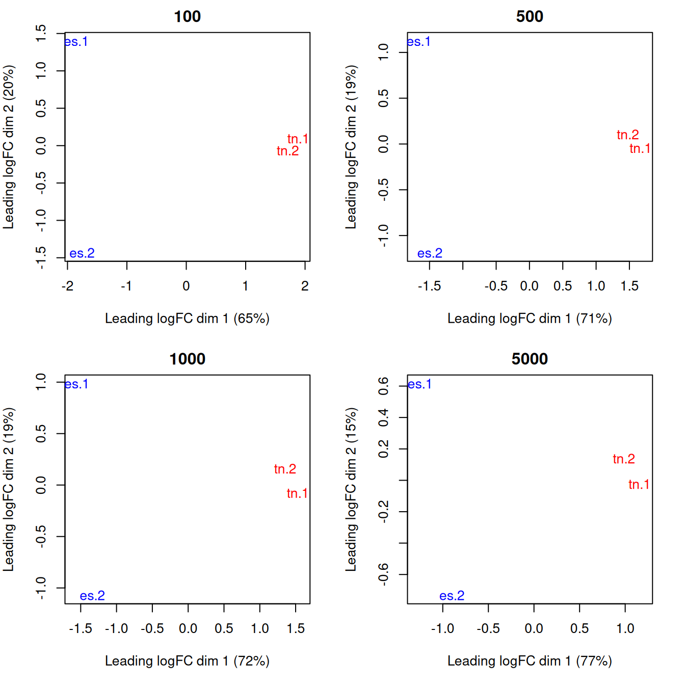
Figure 6.3: MDS plots computed with varying numbers of top windows with the strongest log-fold changes between libaries. In each plot, each library is marked with its name and colored according to its cell type.
Replicates from different groups should form separate clusters in the MDS plot, as observed above. This indicates that the results are reproducible and that the effect sizes are large. Mixing between replicates of different conditions indicates that the biological difference has no effect on protein binding, or that the data is too variable for any effect to manifest. Any outliers should also be noted as their presence may confound the downstream analysis. In the worst case, outlier samples may need to be removed to obtain sensible results.
Session information
R version 4.6.0 RC (2026-04-17 r89917)
Platform: x86_64-pc-linux-gnu
Running under: Ubuntu 24.04.4 LTS

Matrix products: default
BLAS:   /home/biocbuild/bbs-3.23-bioc/R/lib/libRblas.so
LAPACK: /usr/lib/x86_64-linux-gnu/lapack/liblapack.so.3.12.0  LAPACK version 3.12.0

locale:
 [1] LC_CTYPE=en_US.UTF-8       LC_NUMERIC=C
 [3] LC_TIME=en_GB              LC_COLLATE=C
 [5] LC_MONETARY=en_US.UTF-8    LC_MESSAGES=en_US.UTF-8
 [7] LC_PAPER=en_US.UTF-8       LC_NAME=C
 [9] LC_ADDRESS=C               LC_TELEPHONE=C
[11] LC_MEASUREMENT=en_US.UTF-8 LC_IDENTIFICATION=C

time zone: America/New_York
tzcode source: system (glibc)

attached base packages:
[1] stats4    stats     graphics  grDevices utils     datasets  methods
[8] base

other attached packages:
 [1] edgeR_4.10.0                limma_3.68.0
 [3] csaw_1.46.0                 SummarizedExperiment_1.42.0
 [5] Biobase_2.72.0              MatrixGenerics_1.24.0
 [7] matrixStats_1.5.0           GenomicRanges_1.64.0
 [9] Seqinfo_1.2.0               IRanges_2.46.0
[11] S4Vectors_0.50.0            BiocGenerics_0.58.0
[13] generics_0.1.4              BiocStyle_2.40.0
[15] rebook_1.22.0

loaded via a namespace (and not attached):
 [1] sass_0.4.10         SparseArray_1.12.0  bitops_1.0-9
 [4] lattice_0.22-9      digest_0.6.39       evaluate_1.0.5
 [7] grid_4.6.0          bookdown_0.46       fastmap_1.2.0
[10] jsonlite_2.0.0      Matrix_1.7-5        graph_1.90.0
[13] BiocManager_1.30.27 XML_3.99-0.23       Biostrings_2.80.0
[16] codetools_0.2-20    jquerylib_0.1.4     abind_1.4-8
[19] cli_3.6.6           CodeDepends_0.6.7   rlang_1.2.0
[22] crayon_1.5.3        XVector_0.52.0      cachem_1.1.0
[25] DelayedArray_0.38.0 yaml_2.3.12         metapod_1.20.0
[28] otel_0.2.0          S4Arrays_1.12.0     tools_4.6.0
[31] dir.expiry_1.20.0   parallel_4.6.0      BiocParallel_1.46.0
[34] locfit_1.5-9.12     Rsamtools_2.28.0    filelock_1.0.3
[37] R6_2.6.1            lifecycle_1.0.5     bslib_0.10.0
[40] Rcpp_1.1.1-1.1      statmod_1.5.1       xfun_0.57
[43] knitr_1.51          htmltools_0.5.9     rmarkdown_2.31
[46] compiler_4.6.0
Bibliography
Chen, Y., A. T. L. Lun, and G. K. Smyth. 2014. “Differential Expression Analysis of Complex RNA-Seq Experiments Using EdgeR.” In Statistical Analysis of Next Generation Sequence Data, edited by S. Datta and D. S. Nettleton. New York: Springer.
Law, C. W., Y. Chen, W. Shi, and G. K. Smyth. 2014. “Voom: precision weights unlock linear model analysis tools for RNA-seq read counts.” Genome Biol. 15 (2): R29.
Lund, S. P., D. Nettleton, D. J. McCarthy, and G. K. Smyth. 2012. “Detecting differential expression in RNA-sequence data using quasi-likelihood with shrunken dispersion estimates.” Stat. Appl. Genet. Mol. Biol. 11 (5).
McCarthy, D. J., Y. Chen, and G. K. Smyth. 2012. “Differential expression analysis of multifactor RNA-Seq experiments with respect to biological variation.” Nucleic Acids Res. 40 (10): 4288–97.
Phipson, B., S. Lee, I. J. Majewski, W. S. Alexander, and G. K. Smyth. 2016. “Robust Hyperparameter Estimation Protects Against Hypervariable Genes and Improves Power to Detect Differential Expression.” Ann. Appl. Stat. 10 (2): 946–63.
Robinson, M. D., and G. K. Smyth. 2008. “Small-sample estimation of negative binomial dispersion, with applications to SAGE data.” Biostatistics 9 (2): 321–32.
Smyth, G. K. 2004. “Linear models and empirical bayes methods for assessing differential expression in microarray experiments.” Stat. Appl. Genet. Mol. Biol. 3: Article 3.