15 Workflow: Visium HD (binned)
15.1 Introduction
Visium HD is a next-generation spatial transcriptomics technology developed by 10x Genomics, designed to provide single-cell resolution spatial gene expression data across entire tissue sections. Commercially available since 2024, Visium HD advanced the platform’s resolution from 55 µm spots to bins of subcellular resolution (2 µm). In this workflow, we will demonstrate common analysis steps with a Visium HD dataset on colorectal cancer (de Oliveira et al. 2025).
15.2 Dependencies
In this demo, we perform deconvolution on 16 µm bins and compare the concordance with results on 8 µm bins, provided by 10x Genomics.
Code
# retrieve dataset from OSF repo
id <- "VisiumHD_HumanColon_Oliveira"
pa <- OSTA.data_load(id)
dir.create(td <- tempfile())
unzip(pa, exdir=td)
# read 8um bins into 'SpatialExperiment'
vhd8 <- TENxVisiumHD(
    spacerangerOut=td,
    processing="filtered",
    format="h5",
    images="lowres",
    bin_size="008") |>
    import()
# use gene symbols as feature names
gs <- rowData(vhd8)$Symbol
rownames(vhd8) <- make.unique(gs)
vhd8
## class: SpatialExperiment
## dim: 18085 545913
## metadata(2): resouces spatialList
## assays(1): counts
## rownames(18085): SAMD11 NOC2L ... MT-ND6 MT-CYB
## rowData names(3): ID Symbol Type
## colnames(545913): s_008um_00301_00321-1 s_008um_00526_00291-1 ...
## s_008um_00353_00477-1 s_008um_00595_00611-1
## colData names(12): barcode in_tissue ... in_cell sample_id
## reducedDimNames(0):
## mainExpName: Gene Expression
## altExpNames(0):
## spatialCoords names(2) : pxl_col_in_fullres pxl_row_in_fullres
## imgData names(4): sample_id image_id data scaleFactorThese data come with bin-level annotations from deconvolution estimates by RCTD (Cable et al. 2022), implemented in spacexr. Specifically, two sets of labels are available that correspond to the most and second most frequent of 38 cell types per bin, respectively:
Code
# retrieve annotations
gz <- "binned_outputs/square_008um/deconvolution.csv.gz"
df <- read.csv(file.path(td, gz), row.names=2)
head(df <- df[complete.cases(df), -1])
## DeconClass DeconLabel1 DeconLabel2
## s_008um_00000_00001-1 singlet Pericytes Endothelial
## s_008um_00000_00017-1 singlet Enteric Glial Enterocyte
## s_008um_00000_00018-1 doublet_uncertain Enteric Glial Tumor II
## s_008um_00000_00019-1 singlet vSM Tuft
## s_008um_00000_00020-1 singlet vSM CD8 Cytotoxic T cell
## s_008um_00000_00023-1 reject Smooth Muscle vSMCode
lab <- grep("Label", names(cd <- colData(vhd8)), value=TRUE)
pal <- hcl.colors(length(unique(unlist(cd[lab]))), "Spectral")
lapply(lab, \(.) {
  plotCoords(vhd8, annotate=., point_size=0.2, point_shape=15) + ggtitle(.)
}) |>
  wrap_plots(nrow=1, guides="collect") &
  scale_color_manual(NULL, values=pal) &
  theme(legend.key.size=unit(0, "lines"))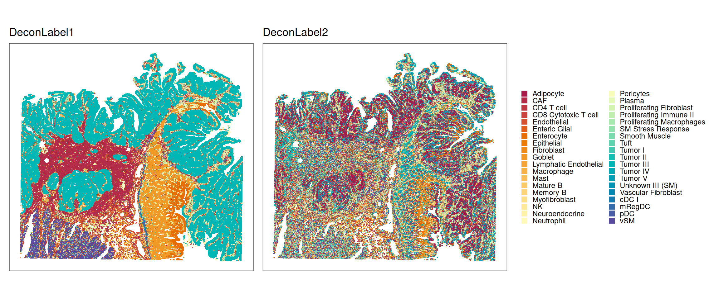
Another resolution of VisiumHD with 16 µm bin can be read in as follow:
Code
# read 16um bins into 'SpatialExperiment'
vhd16 <- TENxVisiumHD(
    spacerangerOut=td,
    processing="filtered",
    format="h5",
    images="lowres",
    bin_size="016") |>
    import()
# use symbols as feature names
gs <- rowData(vhd16)$Symbol
rownames(vhd16) <- make.unique(gs)
vhd16
## class: SpatialExperiment
## dim: 18085 137051
## metadata(2): resouces spatialList
## assays(1): counts
## rownames(18085): SAMD11 NOC2L ... MT-ND6 MT-CYB
## rowData names(3): ID Symbol Type
## colnames(137051): s_016um_00052_00082-1 s_016um_00010_00367-1 ...
## s_016um_00037_00193-1 s_016um_00144_00329-1
## colData names(12): barcode in_tissue ... in_cell sample_id
## reducedDimNames(0):
## mainExpName: Gene Expression
## altExpNames(0):
## spatialCoords names(2) : pxl_col_in_fullres pxl_row_in_fullres
## imgData names(4): sample_id image_id data scaleFactorSome global filtering based on library size is necessary to remove bins that overlay empty tissue.
We can visualize such bins by zooming into an empty tissue region. On the left-hand side, one region shows a clear gap with low counts. Informed by H&E staining, bins located above tissue gaps should not be interpreted biologically, as the low counts in these bins are likely due to ambient RNA or transcript spillover. Therefore, they should be excluded from downstream analysis.
Based on a discussion with the original author at 10x Genomics, in this dataset, 8 µm bins with a library size below 100 are removed. Since we expect a 4-fold increase in library size across all bins at 16 µm, we can set the filtering threshold to 400.
Code
p1 <- plotVisium(vhd16,
    annotate="libsize", point_shape=22,
    zoom=TRUE, show_axes=TRUE, point_size=1.3) +
    xlim(c(422, 442)) + ylim(c(318, 330)) +
    ggtitle("16 µm - original")

vhd16 <- vhd16[, vhd16$libsize > 400]

p2 <- plotVisium(vhd16,
    annotate="libsize", point_shape=22,
    zoom=TRUE, show_axes=TRUE, point_size=1.3) +
    xlim(c(422, 442)) + ylim(c(318, 330)) +
    ggtitle("16 µm - post > 400 UMI QC")

p1 | p2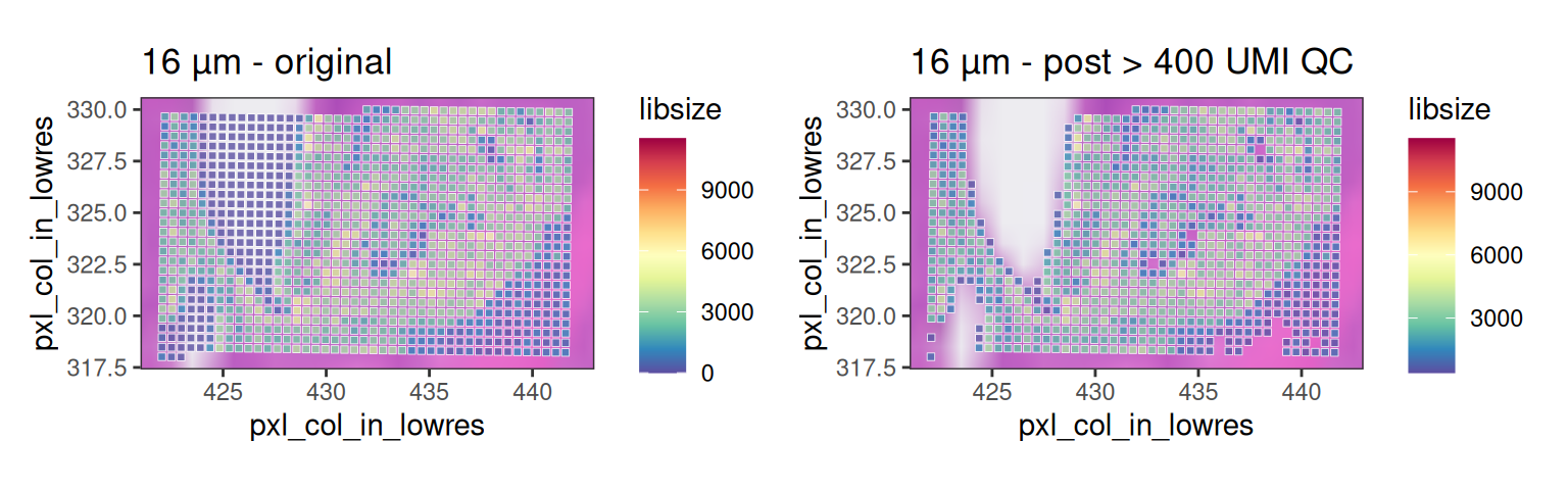
Clustering results generated by Space Ranger are provided for both resolutions.
We can visualize the given clustering results at 8 µm and 16 µm resolutions. Later, we will compare the clustering result at 16 µm with that from Banksy.
Code
(plotCoords(vhd8,
    annotate="cluster", point_size=0.05, point_shape=15,
    pal=unname(pals::kelly())) + ggtitle("8 µm")) |
(plotCoords(vhd16[, !is.na(vhd16$cluster)],
    annotate="cluster", point_size=0.1, point_shape=15,
pal=unname(pals::kelly())) + ggtitle("16 µm")) 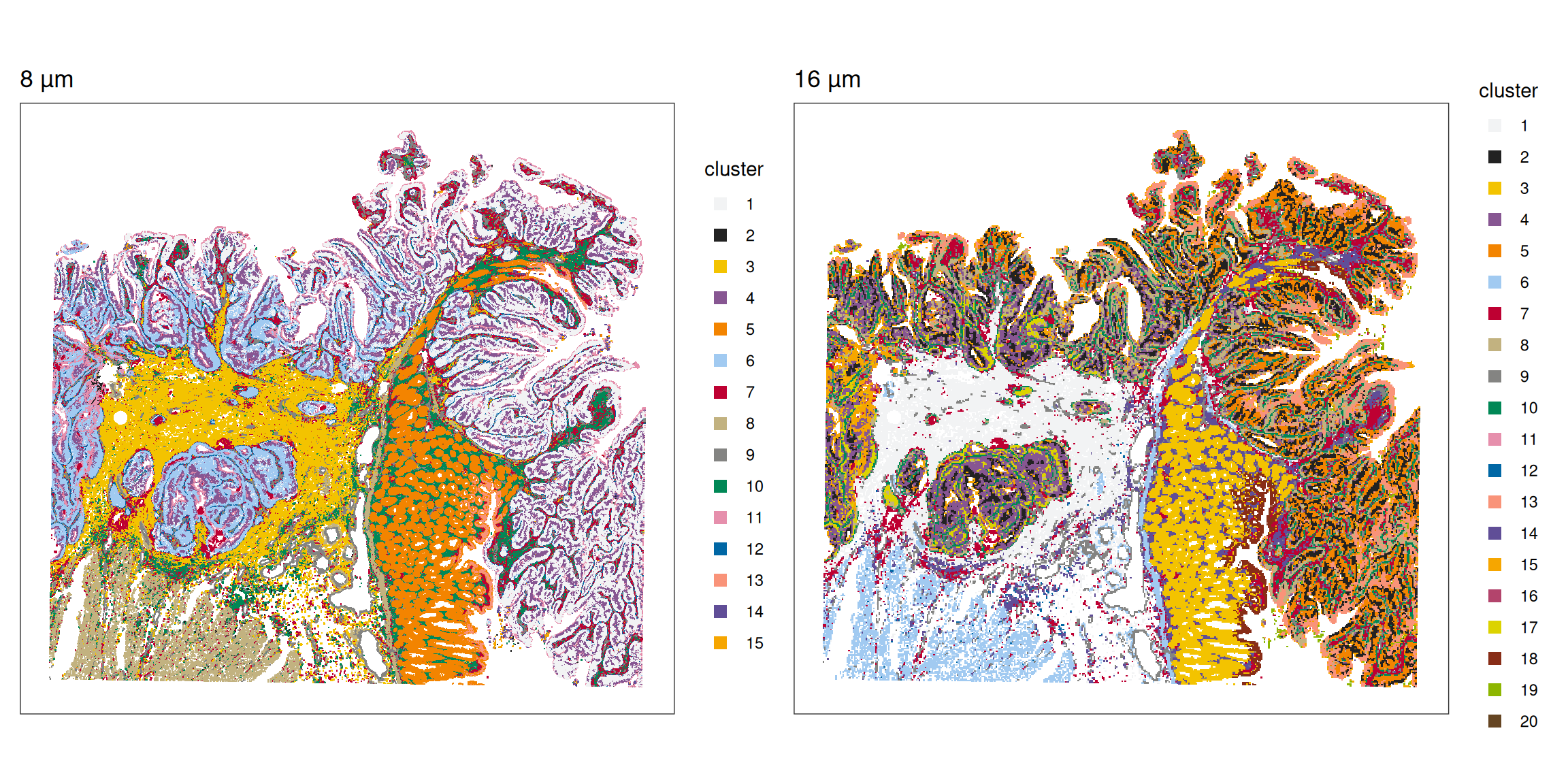
To keep runtimes low, our downstream analysis will be performed on a subset area of 16 µm bins (1/64 of the data coverage area), which we read in here; there are no annotations available for this resolution in the public domain.
Code
.rng <- \(spe) {
    xy <- spatialCoords(spe)*scaleFactors(spe)
    xs <- range(xy[, 1]); ys <- nrow(imgRaster(spe))-range(xy[, 2])
    x1 <- xs[1] + 4*(xs[2]-xs[1])/8; x2 <- xs[2] - 3*(xs[2]-xs[1])/8
    y1 <- ys[1] + 3*(ys[2]-ys[1])/8; y2 <- ys[2] - 4*(ys[2]-ys[1])/8
    list(box=c(x1, x2, y1, y2), cov=c(xs, ys))
}
vhd8r <- .rng(vhd8)
# vhd16r <- .rng(vhd16)
# use 8um bounding boxes to subset spes at both resolutions;
# it is similar to 16um's box range
.box <- \(roi, lty, lwd, col) {
    geom_rect(
        xmin=vhd8r[[roi]][1], xmax=vhd8r[[roi]][2],
        ymin=vhd8r[[roi]][3], ymax=vhd8r[[roi]][4],
        col=col, fill=NA, linetype=lty, linewidth=lwd)
}
cov <- .box(roi="cov", lty=2, lwd=1/2, col="grey")
box <- .box(roi="box", lty=4, lwd=2/3, col="black")
# plotting
.lim <- \(spe) list(
    xlim(spe[["box"]][c(1, 2)]),
    ylim(spe[["box"]][c(4, 3)]))

plotVisium(vhd8, spots=FALSE, point_shape=22) + cov + box +
    ggtitle("grey: data coverage\n black: zoomed region") +
plotVisium(vhd8, point_size=0.8, zoom=TRUE, point_shape=22) + .lim(vhd8r) +
    ggtitle("8 µm bins in black box") +
plotVisium(vhd16, point_size=1.6, zoom=TRUE, point_shape=22) + .lim(vhd8r) +
    ggtitle("16 µm bins in black box") +
plot_layout(nrow=1, widths=c(1.5, 1, 1)) & facet_null() &
    theme(plot.title=element_text(hjust=0.5, vjust=0.5))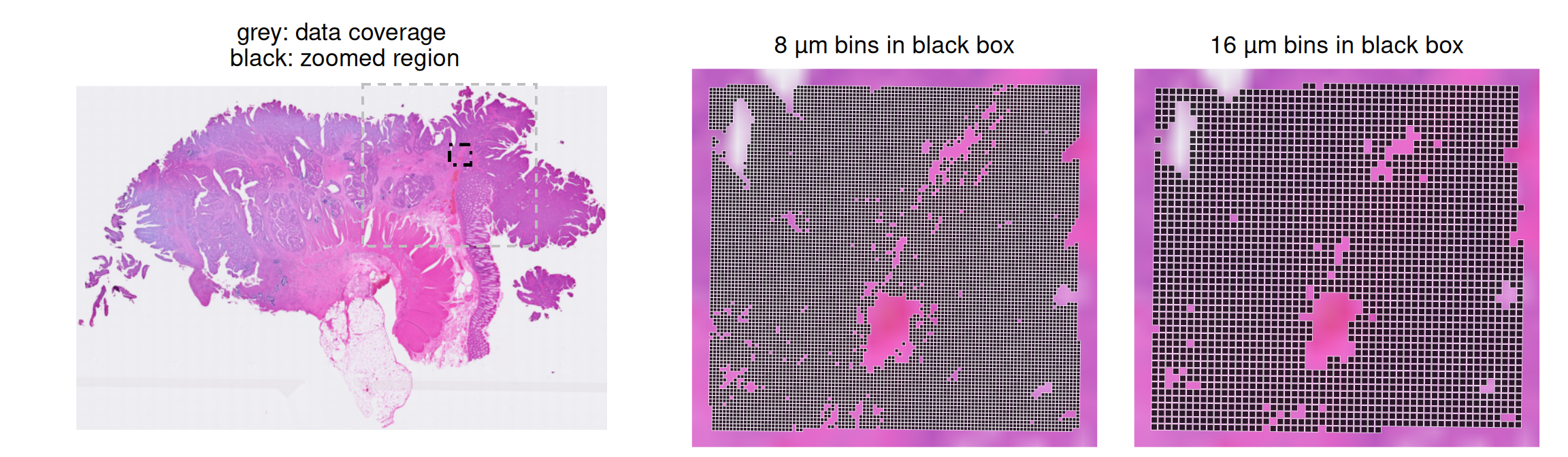
Code
# helper for subsetting
.sub <- function(spe, rng, roi="box") {
    xs <- rng[[roi]][c(1, 2)]
    ys <- nrow(imgRaster(spe)) - rng[[roi]][c(3,4)]
    xy <- spatialCoords(spe)*scaleFactors(spe)
    spe[, xy[, 1] > xs[1] & xy[, 1] < xs[2] &
          xy[, 2] > ys[1] & xy[, 2] < ys[2] ]
}
Subset the 16 µm object to bins in the black box:
Code
.vhd16 <- .sub(spe=vhd16, rng=vhd8r)
dim(.vhd16)
## [1] 18085 2416From now on, we are operating on 2416 16 µm bins.
15.3 Quality control
As detailed in Chapter 10, we use SpotSweeper to perform quality control on the subsetted 16 µm data.
Code
# calculate per-bin QC metrics
mt <- grepl("^MT-", rownames(.vhd16))
.vhd16 <- quickRnaQc.se(.vhd16, subsets=list(mt=mt))
# determine outliers based on
# - low log-library size
# - few uniquely detected features
# - high mitochondrial count proportion
.vhd16 <- localOutliers(.vhd16, metric="sum", direction="lower", log=TRUE)
.vhd16 <- localOutliers(.vhd16, metric="detected", direction="lower", log=TRUE)
.vhd16 <- localOutliers(.vhd16, metric="subset.proportion.mt", direction="higher", log=FALSE)
.vhd16$discard <-
    .vhd16$sum_outliers |
    .vhd16$detected_outliers |
    .vhd16$subset.proportion.mt_outliers
# tabulate number of bins retained
# vs. removed by any criterion
table(.vhd16$discard)
##
## FALSE TRUE
## 2398 18Code
plotCoords(.vhd16, annotate="sum_log", point_size=0.2, point_shape=15) +
  ggtitle("log-library size") +
  plotCoords(.vhd16, annotate="subset.proportion.mt", point_size=0.2, point_shape=15) +
  ggtitle("mitochondrial proportion") +
  plot_layout(nrow=1) & theme(
    legend.key.width=unit(0.5, "lines"),
    legend.key.height=unit(1, "lines")) &
  scale_color_gradientn(colors=pals::jet())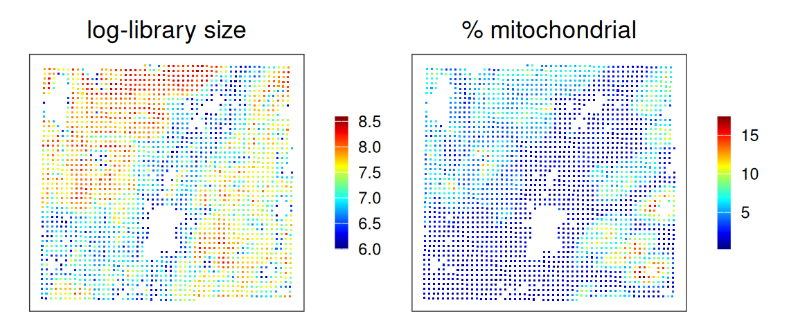
We can visualize the local outliers identified by SpotSweeper in space:
Code
plotCoords(.vhd16, point_shape=15, annotate="discard") + ggtitle("discard") +
plotCoords(.vhd16, point_shape=15, annotate="sum_outliers") + ggtitle("low_lib_size") +
plotCoords(.vhd16, point_shape=15, annotate="detected_outliers") + ggtitle("low_n_features") +
plot_layout(nrow=1, guides="collect") &
    theme(
        plot.title=element_text(hjust=0.5),
        legend.key.size=unit(0, "lines")) &
    guides(col=guide_legend(override.aes=list(size=3))) &
    scale_color_manual("discard", values=c("lavender", "purple"))
Lastly, we subset the Visium HD 16 µm object to bins that passed QC:
Code
.vhd16 <- .vhd16[, !.vhd16$discard]
dim(.vhd16)
## [1] 18085 239815.4 Clustering
First, we identify highly variable genes (HVGs) in the target area:
Code
.vhd16 <- normalizeRnaCounts.se(.vhd16)
.vhd16 <- chooseRnaHvgs.se(
    .vhd16, top=3e3,
    more.var.args=list(use.min.width=TRUE))
hvg <- rownames(.vhd16)[rowData(.vhd16)$hvg]
As detailed in Chapter 28, Banksy (Singhal et al. 2024) utilizes a pair of spatial kernels to capture gene expression variation, followed by dimension reduction and graph-based clustering to identify spatial domains.
Code
# set seed for random number generation
# in order to make results reproducible
set.seed(112358)
# 'Banksy' parameter settings
k <- 8   # consider first order neighbors
l <- 0.2 # use little spatial information
a <- "logcounts"
xy <- c("array_row", "array_col")
# restrict to selected features
tmp <- .vhd16[hvg, ]
# compute spatially aware 'Banksy' PCs
tmp <- computeBanksy(tmp, assay_name=a, coord_names=xy, k_geom=k)
tmp <- runBanksyPCA(tmp, lambda=l, npcs=20)
reducedDim(.vhd16, "PCA") <- reducedDim(tmp)
## run UMAP (for visualization purposes only)
# .vhd16 <- runUmap.se(.vhd16, reddim.type="PCA")
# build cellular shared nearest-neighbor (SNN) graph
# and cluster using Leiden community detection algorithm
.vhd16 <- clusterGraph.se(
    .vhd16, num.neighbors=20,
    method="leiden", resolution=1.2,
    more.build.args=list(weight.scheme="jaccard"),
    more.cluster.args=list(leiden.objective="modularity", seed=112358),
    reddim.type="PCA", output.name="Banksy")
table(.vhd16$Banksy)
##
## 1 2 3 4 5 6 7 8 9 10 11 12 13 14
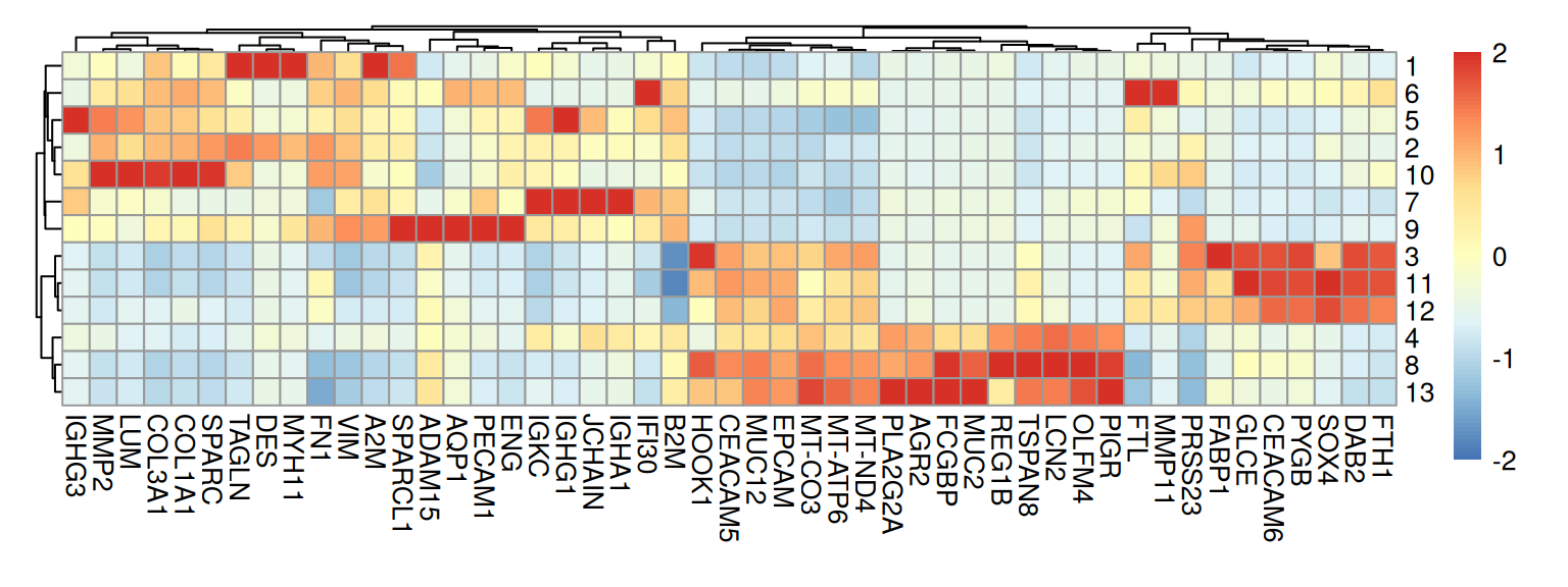
## 156 197 174 196 224 183 229 71 127 276 180 208 88 89Next, we can score marker genes for each cluster; c.f. Chapter 30. We also compute the cluster-wise mean expression of selected markers:
Code
# marker gene scoring
mgs <- scoreMarkers.se(.vhd16, groups=.vhd16$Banksy)
# select for a few markers per cluster
top <- lapply(mgs, \(df) rownames(df)[df$cohens.d.min.rank <= 2])
top <- unique(unlist(top))
# average expression by clusters
pbs <- aggregateAcrossCells.se(
    .vhd16[top, ], factors=.vhd16$Banksy, assay.type="logcounts")
means <- t(t(assay(pbs, "sums")) / pbs$counts)
The marker genes in each cluster can be visualized with a heatmap:
Code
Or, we can visualize the bin-wise expression of selected markers in space:
Code
gs <- c("MMP2", "PIGR", "IGHG1")
ps <- lapply(gs, \(.) plotCoords(.vhd16, annotate=., point_shape=15,
                                 point_size=0.8, assay_name="logcounts"))
wrap_plots(ps, nrow=1) & theme(
  legend.key.width=unit(0.5, "lines"),
  legend.key.height=unit(1, "lines")) &
  scale_color_gradientn(colors=rev(hcl.colors(9, "Rocket")))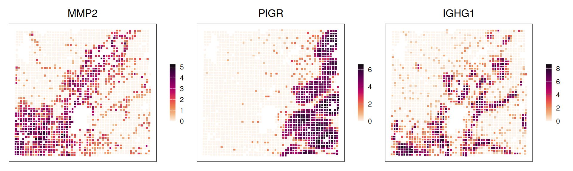
15.5 Deconvolution
15.5.1 Load single-cell reference
We will now perform deconvolution on the 16 µm binned Visium HD data. First, we retrieve matching (Chromium) scRNA-seq data, which includes low- (Level1) and high-resolution (Level2) annotations of cells into 9 respectively 31 clusters. In order to ensure similar transcriptional profile across technologies, we filter the reference population to patient 2 only.
Code
# retrieve dataset from OSF repository
id <- "Chromium_HumanColon_Oliveira"
pa <- OSTA.data_load(id)
dir.create(td <- tempfile())
unzip(pa, exdir=td)
# read into `SingleCellExperiment`
fs <- list.files(td, full.names=TRUE)
h5 <- grep("h5$", fs, value=TRUE)
sce <- read10xCounts(h5, col.names=TRUE)
# add cell metadata
csv <- grep("csv$", fs, value=TRUE)
cd <- read.csv(csv, row.names=1)
colData(sce)[names(cd)] <- cd[colnames(sce), ]
# use gene symbols as feature names
gs <- rowData(sce)$Symbol
rownames(sce) <- make.unique(gs)
# exclude cells deemed to be of low-quality
sce <- sce[, sce$QCFilter == "Keep"]
# subset cells from same patient
sce <- sce[, grepl("P2", sce$Patient)]
sce
## class: SingleCellExperiment
## dim: 18082 67568
## metadata(1): Samples
## assays(1): counts
## rownames(18082): SAMD11 NOC2L ... MT-ND6 MT-CYB
## rowData names(3): ID Symbol Type
## colnames(67568): AAACAAGCAACAGCTAACTTTAGG-1
## AAACAAGCAACTGTTCACTTTAGG-1 ... TTTGTGAGTGCGTACCATGTTGAC-24
## TTTGTGAGTGGAAGCTATGTTGAC-24
## colData names(7): Sample Barcode ... Level1 Level2
## reducedDimNames(0):
## mainExpName: NULL
## altExpNames(0):We can visualize the mapping between low- and high-resolution annotations in the single-cell reference data with a contingency table:
Code
fq <- prop.table(table(sce$Level1, sce$Level2), 2)
pheatmap(fq, cellwidth=10, cellheight=10, treeheight_row=5, treeheight_col=5)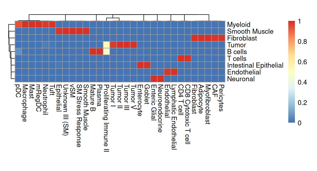
Note that "Proliferating Immune II" spans evenly between "B cells" and "Tumor", so we will make it a separate class, "Prolif. Immune" in the low-resolution annotations:
Code
##
##                B cells           Endothelial            Fibroblast
##                   6233                  1969                  7355
##  Intestinal Epithelial               Myeloid              Neuronal
##                   5949                  6353                  1216
##         Prolif. Immune         Smooth Muscle               T cells
##                    810                 16428                  6658
##                  Tumor
##                  14597
There are some differences in the provided deconvolution labels at 8 µm resolution and the high-resolution single-cell reference labels:
Code
# all single-cell reference labels
# are present in the Visium HD data
setdiff(sce$Level2, vhd8$DeconLabel1)
## character(0)Code
setdiff(sce$Level2, vhd8$DeconLabel2)## character(0)Code
# but not vice versa
setdiff(vhd8$DeconLabel1, sce$Level2)
## [1] "Proliferating Macrophages" "Proliferating Fibroblast"
## [3] "Memory B" "Vascular Fibroblast"
## [5] "cDC I" "NK"
## [7] "Tumor IV"Code
setdiff(vhd8$DeconLabel2, sce$Level2)## [1] "Proliferating Fibroblast" "Memory B"
## [3] "cDC I" "Proliferating Macrophages"
## [5] "Vascular Fibroblast" "Tumor IV"
## [7] "NK"Below, these extra classes in the Visium HD 8 μm bin annotations will be ignored.
15.5.2 Simplify 8 µm annotations
We can merge the provided deconvolution annotation "DeconLabel1" (most likely cell type for singlets, most dominant type for doublets) into a lower resolution using the single-cell reference annotations:
Code
##
##                B cells           Endothelial            Fibroblast
##                  12279                 19978                 75080
##  Intestinal Epithelial               Myeloid              Neuronal
##                  40683                 20811                  1200
##         Prolif. Immune         Smooth Muscle               T cells
##                   3660                 15913                  6158
##                  Tumor
##                 215865
According to RCTD, approximately 75% of the 8 µm bins are singlets:
Let us check the top-5 common doublet pairs according to the "doublet_certain" class:
Code
dbl <- vhd8$DeconClass == "doublet_certain"
lab <- c(".DeconLabel1", ".DeconLabel2")
df <- data.frame(colData(vhd8)[dbl, lab])
# sort as to ignore order
df <- apply(df, 1, sort)
df <- do.call(rbind, df)
names(df) <- lab
# count unique pairs
ij <- paste(df[, 1], df[, 2], sep=";")
head(sort(table(ij), decreasing=TRUE), 5)
## ij
## Myeloid;Tumor B cells;Fibroblast Fibroblast;Myeloid Tumor;Tumor
## 3799 3670 3453 2742
## Fibroblast;Tumor
## 2532We can see that myeloid are commonly co-localized with tumor and fibroblasts cells; most doublets are homotypic, i.e., they are (mostly) composed of one low-resolution type.
We can perform the same subsetting procedure to 8 µm bins and compare the difference in the number of bins in the zoomed (black box) area.
Code
# subset zoomed (black box) area
.vhd8 <- .sub(spe=vhd8, rng=vhd8r)
# compare number of bins between resolutions
(n <- ncol(.vhd8))
## [1] 8933Code
(m <- ncol(.vhd16))## [1] 2398Code
round(n/m, 2)## [1] 3.73As expected, the number of 8 µm bins is about 4 times the number of 16 µm bins. We will visualize the same subset for both bin sizes in any downstream analyses.
15.5.3 Run RCTD on 16 µm bins
We also assume there are at most two cell types in a 16 µm bin as in 8 µm, and thus we would expect a smaller proportion of singlets.
Code
# downsample to at most 4,000 cells per cluster for 'sce'
# (this is done only to keep runtime/memory low)
cs <- split(seq_len(ncol(sce)), sce$Level1)
cs <- lapply(cs, \(.) sample(., min(length(.), 4e3)))
ncol(.sce <- sce[, unlist(cs)])
rctd_data <- createRctd(.vhd16, .sce, cell_type_col="Level1")
(res <- runRctd(rctd_data, max_cores=4, rctd_mode="doublet"))
Weights inferred by RCTD correspond to proportions of cell types, such that they sum to 1 for a given observation (expect for rejected ones, which sum to 0):
##
##  FALSE  TRUE
##   2388    10
Code
# add proportion estimates as metadata
ws <- data.frame(t(as.matrix(ws)))
colData(.vhd16)[names(ws)] <- ws[colnames(.vhd16), ]
Next, we can spatially visualize the deconvolution proportions estimates:
Code
lapply(names(ws), \(.)
    plotCoords(.vhd16, annotate=., point_size=0.3, point_shape=15)) |>
    wrap_plots(nrow=2, guides="collect") & theme(
    legend.key.width=unit(0.5, "lines"),
    legend.key.height=unit(1, "lines")) &
    scale_color_gradientn(colors=rev(hcl.colors(9, "Rocket")))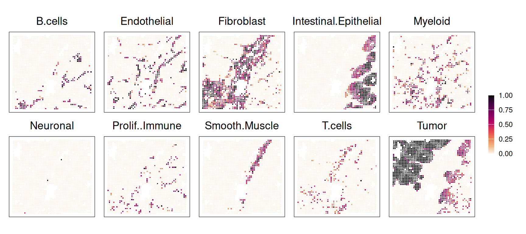
We may also obtain the majority vote class for 16 µm bins:
Code
##
##                B cells           Endothelial            Fibroblast
##                    119                   227                   504
##  Intestinal Epithelial               Myeloid              Neuronal
##                    371                   181                     2
##         Prolif. Immune         Smooth Muscle               T cells
##                     81                    56                    48
##                  Tumor
## 809We can also check the proportional frequency difference between 8 and 16 µm bins in our region of interest:
Code
n8 <- table(.vhd8$.DeconLabel1)
n16 <- table(.vhd16$.DeconLabel1)
df <- data.frame(x=as.numeric(n8/n16))
ggplot(df, aes(x)) + geom_density() +
    xlab("Cell type frequency ratio") +
    ggtitle("distribution of cell type frequency\nratio between 8 vs. 16 µm bins") +
    scale_x_continuous(breaks=seq(0, max(df$x), by=2)) +
    theme_classic() + theme(plot.title=element_text(hjust=0.5))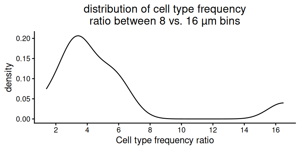
Most cell types appear around 3-4 times more in 8 compared to 16 µm bins, which is expected given the difference in bin size.
15.5.4 Deconvolution results at different resolutions
Let’s visualize deconvolution result for 8 and 16 µm bins in the zoomed area:
Code
plotVisium(.vhd8,
    annotate=".DeconLabel1", zoom=TRUE,
    point_size=0.8, point_shape=22) +
    ggtitle("8 µm") +
plot_spacer() +
plotVisium(.vhd16,
    annotate=".DeconLabel1", zoom=TRUE,
    point_size=1.6, point_shape=22) +
    ggtitle("16 µm") +
plot_layout(nrow=1, guides="collect", widths=c(1, 0.05, 1)) &
    guides(col=guide_legend(override.aes=list(size=2))) &
    scale_fill_manual(values=unname(pals::trubetskoy())) &
    facet_null() & theme(
        plot.title=element_text(hjust=0.5),
legend.key.size=unit(0, "lines")) 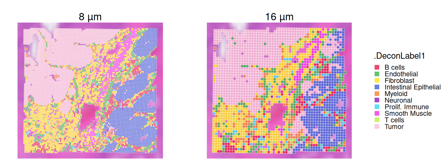
We observe clear agreement in deconvolution at both 8 µm and 16 µm resolutions; however, the 8 µm resolution better captures fine structures, such as the string-like shape of endothelial and fibroblast bins extending into the upper left tumor region.
15.6 Concordance of results
We can visualize the results spatially:
Code
plotVisium(.vhd16,
    annotate="cluster", zoom=TRUE,
    point_shape=22, point_size=1.6,
    pal=unname(pals::kelly())) +
plot_spacer() +
plotVisium(.vhd16,
    annotate="Banksy", zoom=TRUE,
    point_shape=22, point_size=1.6,
    pal=unname(pals::kelly())) +
plot_spacer() +
plotVisium(.vhd16,
    annotate=".DeconLabel1", zoom=TRUE,
    point_shape=22, point_size=1.6,
    pal=unname(pals::trubetskoy())) +
plot_layout(nrow=1, widths=c(1, 0.05, 1, 0.05, 1)) &
    facet_null() & theme(legend.key.size=unit(0, "lines"))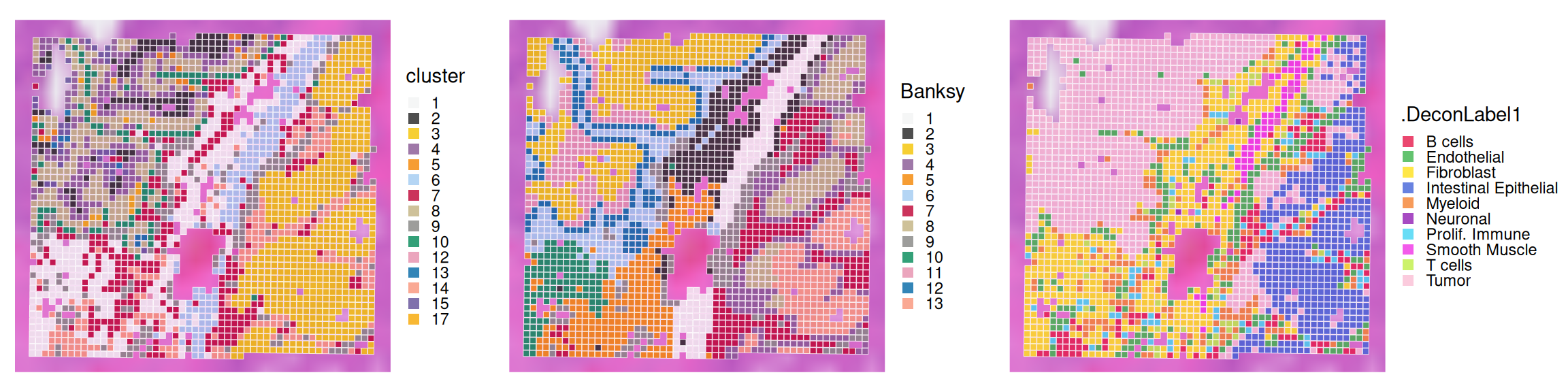
We observe that Banksy delineates tissue borders very well, while deconvolution provides direct biological insight into the underlying clusters. Their concordance can be visualized using a heatmap:
Code
fq <- prop.table(table(.vhd16$Banksy, .vhd16$.DeconLabel1), 1)
pheatmap(fq, cellwidth=10, cellheight=10, treeheight_row=5, treeheight_col=5)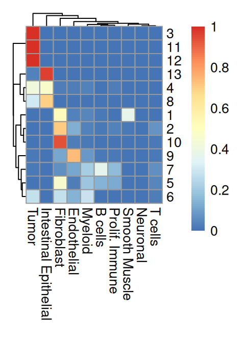
From the above heatmap, cluster 5 and 7 are mostly immune cells; cluster 9 maps to endothelial; cluster 1 and 13 correspond to intestinal epithelial and smooth muscle cells, respectively; fibroblasts map to cluster 10; tumor spans clusters 3, 11 and 12.
15.7 Neighborhood analysis
Here, we want to quantify the abundance between T cells, B cells, or Myeloid bins to Fibroblast or Tumor bins in 8 µm zoomed region. We use getAbundances() from Statial (Ameen et al. 2024) to calculate, for each bin, the abundance of other cell types within a radius of 200 px; the resulting (bins \(\times\) types) matrix is stored as reducedDim slot "abundances".
Code
# check for availability of 'Statial';
# disable coming chunks if unavailable
run <- require("Statial", quietly=TRUE)
if (!run) knitr::opts_chunk$set(eval=FALSE)
Code
.vhd8 <- .vhd8[, !is.na(.vhd8$.DeconLabel1)]
xy <- data.frame(spatialCoords(.vhd8))
colData(.vhd8)[names(xy)] <- xy
.vhd8 <- getAbundances(.vhd8,
    spatialCoords=names(xy),
    cellType=".DeconLabel1",
    imageID="sample_id",
    r=200, nCores=4)
Let’s have a look at the abundance and distance results, also including deconvolution results:
Code
df <- reducedDim(.vhd8, "abundances")
df$CT <- .vhd8$.DeconLabel1
df[1:5, 1:5]
## Fibroblast T cells B cells Prolif. Immune Myeloid
## s_008um_00388_00417-1 38 0 3 0 1
## s_008um_00388_00418-1 43 0 3 1 0
## s_008um_00388_00419-1 44 0 4 1 1
## s_008um_00388_00420-1 47 0 8 1 1
## s_008um_00388_00421-1 50 0 11 1 1Now, we filter to only T cells, B cells and Myeloid bins, and investigate – within their neighborhood – the spatial proximity differences to Fibroblast or Tumor bins in terms of abundance.
Code
source <- df$CT %in% c("T cells", "B cells", "Myeloid")
target <- c("Tumor", "Fibroblast", "CT")
fd <- pivot_longer(
    df[source, target], cols=-CT,
    names_to="target", values_to="n")
head(fd)
## # A tibble: 6 × 3
## CT target n
## <chr> <chr> <int>
## 1 Myeloid Tumor 0
## 2 Myeloid Fibroblast 43
## 3 B cells Tumor 0
## 4 B cells Fibroblast 50
## 5 B cells Tumor 0
## 6 B cells Fibroblast 50In this region, we observe more fibroblast than tumor bins around each of the immune bins. However, note that in this zoomed region, we have nearly 1.4 times more fibroblast bins compared to tumor bins. Thus, we need to scale abundance values by the number of target cell type bins observed in the region.
Code
n_tum <- table(.vhd8$.DeconLabel1)["Tumor"]
n_fib <- table(.vhd8$.DeconLabel1)["Fibroblast"]
fd$p <- ifelse(fd$target == "Tumor", fd$n/n_tum, fd$n/n_fib)
ggplot(fd, aes(x=CT, y=n, fill=target)) +
    labs(y="# cells within 200px") +
ggplot(fd, aes(x=CT, y=p, fill=target)) +
    labs(y="relative abundance") +
plot_layout(nrow=1, guides="collect") &
    geom_boxplot(key_glyph="point") &
    scale_fill_manual(values=c("yellow", "pink")) &
    guides(fill=guide_legend(override.aes=list(shape=21, size=2))) &
    theme_classic() & theme(
        axis.title.x=element_blank(),
        legend.key.size=unit(0, "lines"))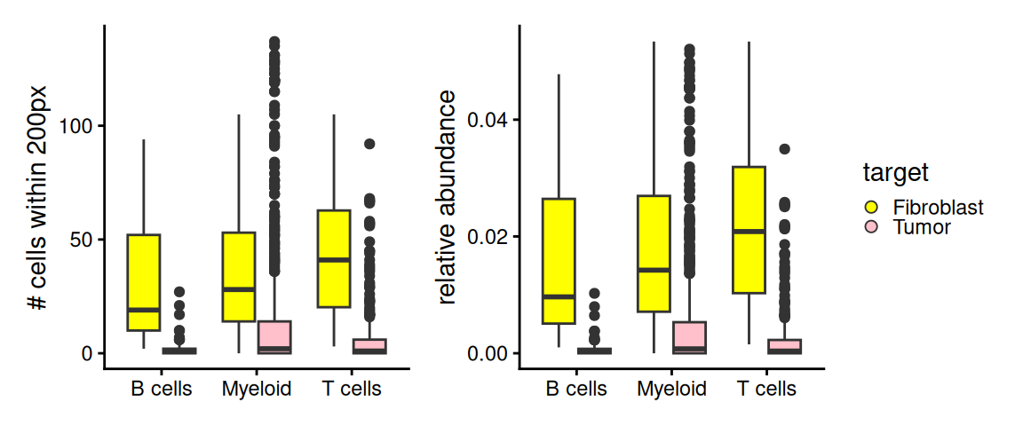
After correction, we see amplified differences in the relative abundance of fibroblast bins compared to tumor bins around each immune cell type in the zoomed region.
We can also investigate the “cell-cell-marker” relationship based on the minimum distance between two cell types within a given radius. The matrix of minimum distance between all pairwise cell types is stored in the reduced dimension, similar to how the abundance matrix was previously stored.
Code
# NOTE: conversion to SCE is a temporary fix for a 'Statial' bug
# reported here: https://github.com/SydneyBioX/Statial/issues/16
tmp <- as(.vhd8, "SingleCellExperiment")
tmp <- getDistances(tmp,
    cellType=".DeconLabel1", imageID="sample_id",
    spatialCoords=names(xy), maxDist=200, nCores=4)
reducedDim(.vhd8, "distances") <- reducedDim(tmp, "distances")
Here, we aim to determine whether the expression level of the tumor marker changes in proximity to fibroblast. Using FTH1 as an example, we observe a decrease in FTH1 expression in tumor bins as the distance to fibroblast increase. This trend could be visualized using a scatter plot.
Code
p <- plotStateChanges(
    cells=.vhd8,
    image="sample01",
    from="Tumor",
    to="Fibroblast",
    marker="FTH1",
    cellType=".DeconLabel1",
    imageID="sample_id",
    spatialCoords=c("array_col", "array_row"))
p$image + facet_null() | p$scatter 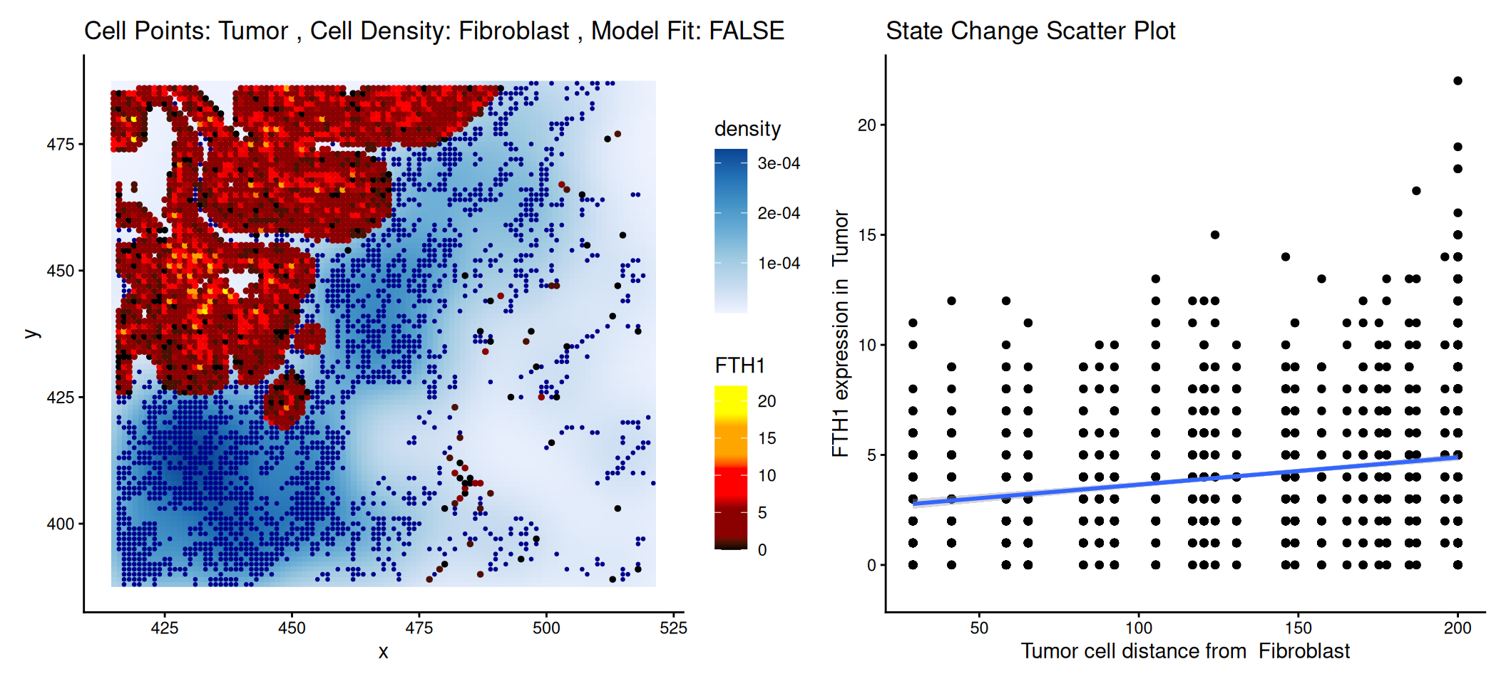
The same analysis steps could be applied to the (unfiltered) 16 μm resolution data with the corresponding deconvolution results.
15.8 Conclusion
In this workflow, we demonstrated how to perform a standard analysis pipeline on a subset of Visium HD data binned at 16 µm. Most methods and visualization techniques developed for Visium can be applied to Visium HD. However, more sparsity is expected, as each data point (e.g. 2, 8, or 16 µm) has smaller area compared to Visium (55 µm). Each bin cannot be interpreted as a cell, but rather, a segmentation-free approach is applied here. Below are some resources for Visium HD to consider and incorporate into your pipeline:
GitHub repository of
bin2cellfor H&E segmentation and obtaining cell boundaries.Analysis pipeline by 10x Genomics (April 2024). The analysis consists of three steps: run
StarDistnuclei segmentation in Python, sum gene expression into nuclei based on segmentation mask, and downstream analysis withscanpyandanndata.Pipeline on cell typing for Visium HD in Python by Sanofi.