11 Intermediate processing

11.1 Preamble

11.1.1 Introduction

This chapter demonstrates methods for several intermediate processing steps – normalization, feature selection, and dimensionality reduction – that are required before downstream analysis methods can be applied.

We use methods from the scrapper Bioconductor package, which were originally developed for scRNA-seq data, with the (simplified) assumption that these methods can be applied to spot-based ST data by treating spots as equivalent to cells. In addition, we discuss alternative spatially-aware methods, and provide links to later parts of the book where these methods are described in more detail.

Following the processing steps, this chapter also includes short demonstrations for subsequent steps, including clustering and identification of marker genes. For more details on these steps, see the later analysis chapters or workflow chapters.

11.1.2 Dependencies

Code

library(scrapper)
library(ggspavis)
library(pheatmap)
library(patchwork)
library(BayesSpace)
library(SpatialExperiment)

Code

# set seed for reproducibility
set.seed(100)

11.1.3 Load data

Here, we load 10x Genomics Visium data from one postmortem human brain tissue section from the dorsolateral prefrontal cortex (DLPFC) brain region (Maynard et al. 2021), which has previously undergone quality control and filtering (see also Chapter 10).

Code

# load data
(spe <- readRDS("seq-spe_qc.rds"))

##  class: SpatialExperiment 
##  dim: 21842 3639 
##  metadata(1): qc
##  assays(1): counts
##  rownames(21842): ENSG00000243485 ENSG00000238009 ... ENSG00000271254
##    ENSG00000268674
##  rowData names(3): gene_id gene_name feature_type
##  colnames(3639): AAACAAGTATCTCCCA-1 AAACAATCTACTAGCA-1 ...
##    TTGTTTGTATTACACG-1 TTGTTTGTGTAAATTC-1
##  colData names(12): barcode_id sample_id ... subset.proportion.mito
##    keep
##  reducedDimNames(0):
##  mainExpName: NULL
##  altExpNames(0):
##  spatialCoords names(2) : pxl_col_in_fullres pxl_row_in_fullres
##  imgData names(4): sample_id image_id data scaleFactor

11.2 Normalization

11.2.1 Library size normalization

A simple and fast approach for normalization is “library size normalization”, which consists of calculating log-transformed normalized counts (“logcounts”) using library size factors, treating each spot as equivalent to a single cell. This method is simple, fast, and generally provides a good baseline. It can be calculated using the scrapper package.

11.2.2 Spatially-aware normalization

SpaNorm (Salim et al. 2025) was developed for ST data, using a gene-wise model (e.g. negative binomial) in which variation is decomposed into a library size-dependent (technical) and -independent (biological) component.

11.3 Feature selection

11.3.1 Highly variable genes (HVGs)

Identifying a set of top “highly variable genes” (HVGs) is a standard step for feature selection in many scRNA-seq workflows, which can also be used as a simple and fast baseline approach in spot-based ST data. This makes the simplified assumption that spots can be treated as equivalent to cells.

Here, we take a standard approach for selecting HVGs; see Section 29.2.1 for more details. We first remove mitochondrial genes, since these tend to be very highly expressed and are not of main biological interest.

Code

# identify mitochondrial genes
nm <- rowData(spe)$gene_name
mt <- grepl("^MT-", nm, ignore.case = TRUE)
table(mt)
# remove them
spe <- spe[!mt, ]

##  mt
##  FALSE  TRUE 
##  21829    13

Next, apply methods from scrapper. This stores the selected HVGs in rowData(spe)$hvg, which can be used as the input for subsequent steps. The argument top defines the number of HVGs to select. Here, we select the top 10% of genes. Alternatively, a fixed number of top HVGs may be selected, say 1000 or 2000.

Code

# fit mean-variance relationship and select top HVGs
spe <- chooseRnaHvgs.se(
    spe, 
    top = ceiling(0.1 * nrow(spe)),
    more.var.args = list(use.min.width = TRUE))

# plot
rd <- rowData(spe)
plot(rd$means, rd$variances, 
    xlab = "mean (logexpr)", ylab = "variance (logexpr)")
o <- order(rd$means)
lines(rd$means[o], rd$fitted[o], col = "dodgerblue")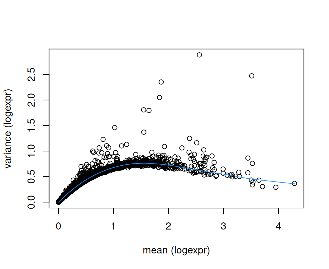

Code

# select top HVGs
sel <- rownames(spe)[rd$hvg]
# number of HVGs selected
length(sel)

##  [1] 2183

11.3.2 Spatially variable genes (SVGs)

Alternatively, spatially-aware methods can be used to identify a set of “spatially variable genes” (SVGs). These methods take the spatial coordinates of the measurements into account, which can generate a more biologically informative ranking of genes associated with biological structure within the tissue area. The set of SVGs may then be used either instead of or complementary to HVGs in subsequent steps.

A number of methods have been developed to identify SVGs. For more details and examples, see Section 29.3.1.

11.4 Dimensionality reduction

A standard next step is to perform dimensionality reduction using principal component analysis (PCA), applied to the set of top HVGs (or SVGs). The set of top principal components (PCs) can then be used as the input for subsequent steps. See Chapter 27 for more details.

Note that we have set a random seed at the start of the chapter for reproducibility.

Code

spe <- runPca.se(spe, features = sel, number = 50)

##  using unknown matrix fallback for 'dgTMatrix'

Code

colnames(reducedDim(spe, "PCA")) <- paste0(
    "PC", seq_len(ncol(reducedDim(spe, "PCA"))))

In addition, we can perform nonlinear dimensionality reduction using the UMAP algorithm, applied to the set of top PCs (default 50). The first two UMAP dimensions can be used for visualization purposes by plotting them on the x and y axes.

Code

spe <- runUmap.se(spe, reddim.type = "PCA")

11.5 Clustering

After completing the intermediate processing steps above, we next demonstrate some short examples of downstream analysis steps.

Here, we run a spatially-aware clustering algorithm, BayesSpace (Zhao et al. 2021), to identify spatial domains. BayesSpace was developed for sequencing-based ST data, and takes the spatial coordinates of the measurements into account.

For more details on clustering, see Chapter 28.

Code

# run BayesSpace clustering
.spe <- spatialPreprocess(spe, skip.PCA = TRUE)
.spe <- spatialCluster(.spe, nrep = 1000, burn.in = 100, q = 10, d = 20)

# cluster labels
table(spe$BayesSpace <- factor(.spe$spatial.cluster))

##  
##    1   2   3   4   5   6   7   8   9  10 
##  253 527 196 314  35 491 270 382 532 639

11.6 Visualizations

We can visualize the cluster labels in x-y space as spatial domains, alongside the manually annotated reference labels (ground_truth) available for this dataset.

Code

# using plotting functions from ggspavis package
# and formatting using patchwork package
plotCoords(spe, annotate = "ground_truth") + 
plotCoords(spe, annotate = "BayesSpace") + 
  plot_layout() & 
  theme(legend.key.size = unit(0, "lines")) & 
  scale_color_manual(values = unname(pals::trubetskoy()))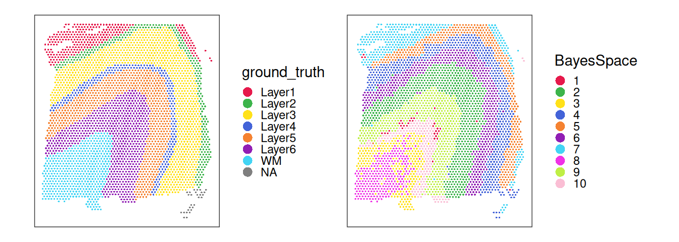

Code

table(spe$BayesSpace, spe$ground_truth, useNA = "ifany")

##      
##       Layer1 Layer2 Layer3 Layer4 Layer5 Layer6  WM <NA>
##    1       1      0      0      0      0     41 211    0
##    2       0      3    454     67      3      0   0    0
##    3       1      0      0      0      0    162  33    0
##    4     268     41      4      0      0      1   0    0
##    5       1      0      0      0      0     33   0    1
##    6       2    207    282      0      0      0   0    0
##    7       0      0      0      0      0      1 269    0
##    8       0      2    249     90     15      0   0   26
##    9       0      0      0      0    101    431   0    0
##    10      0      0      0     61    554     23   0    1

Inspecting the spatial distribution of the top PCs, we can observe that the main driver of expression variability is the distinction between white matter (WM) and non-WM cortical layers.

Code

pcs <- reducedDim(spe, "PCA")
pcs <- pcs[, seq_len(4)]
lapply(colnames(pcs), \(.) {
    spe[[.]] <- pcs[, .]
    plotCoords(spe, annotate = .)
}) |> 
    wrap_plots(nrow = 1) & coord_equal() & 
    geom_point(shape = 16, stroke = 0, size = 0.2) & 
    scale_color_gradientn(colors = pals::jet(), n.breaks = 3) & 
    theme_void() & theme(
        plot.title = element_text(hjust = 0.5), 
        legend.key.width = unit(0.2, "lines"), 
        legend.key.height = unit(0.8, "lines"))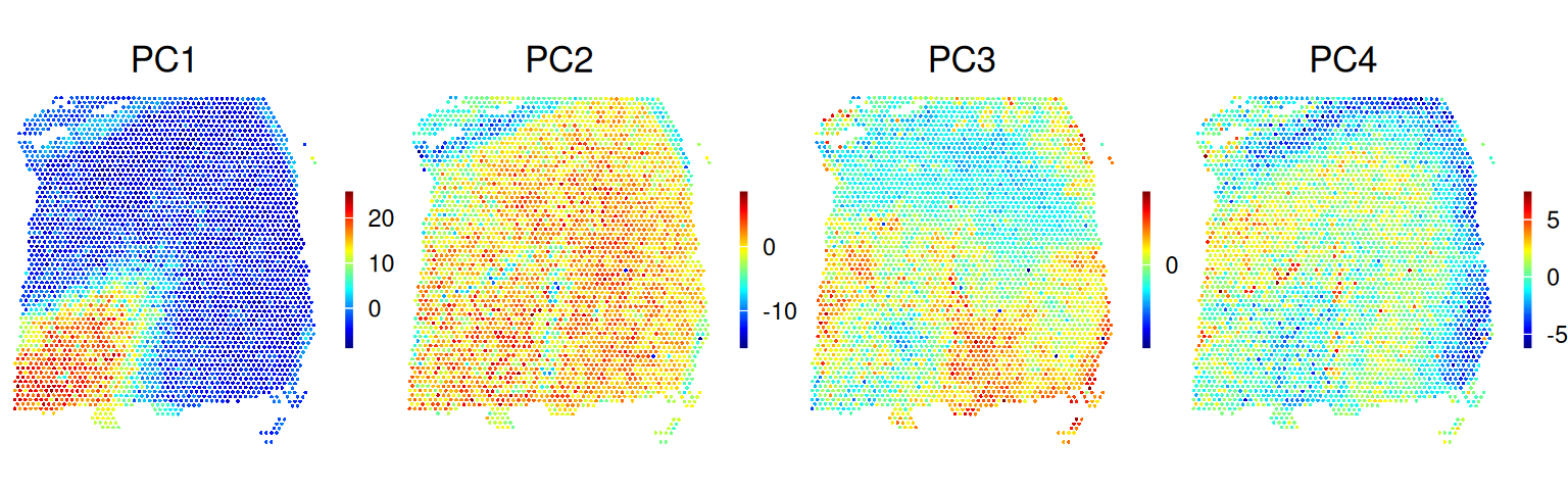

11.7 Marker genes

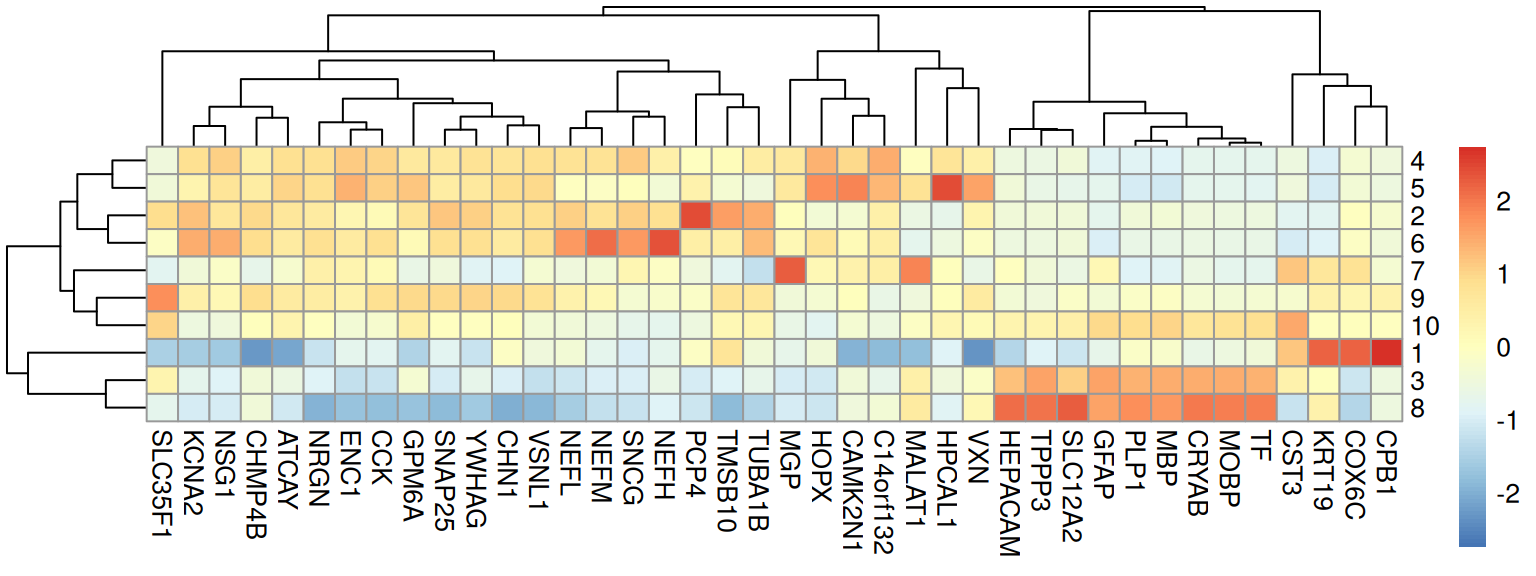
Having clustered our spots to identify spatial domains, we can identify genes with elevated expression in each spatial domain, which can be interpreted as marker genes for the spatial domains; see also Section 29.2.2.

Here, we score candidate marker genes using pairwise effect sizes, i.e. expression should be higher in the cluster for which a gene is reported to be a marker. See Chapter 28 for additional details.

Alternatively, we could also test for spatially variable genes (SVGs) within domains to identify genes with spatial expression patterns that vary independently of the spatial arrangement of domains; see Section 29.3.1 for details.

Code

# using scrapper package
mgs <- scoreMarkers.se(spe, groups = spe$BayesSpace)

##  using unknown matrix fallback for 'dgTMatrix'

Code

top <- lapply(mgs, \(df) rownames(df)[df$cohens.d.min.rank <= 2])
length(top <- unique(unlist(top)))

##  [1] 37

We can visualize selected markers as a heatmap (of cluster-wise expression means):

Code

# compute cluster-wise averages
pbs <- aggregateAcrossCells.se(
    spe[top, ], factors = spe$BayesSpace, assay.type = "logcounts")

##  using unknown matrix fallback for 'dgTMatrix'

Code

means <- t(t(assay(pbs, "sums")) / pbs$counts)

# use gene symbols as feature names
mtx <- t(means)
colnames(mtx) <- rowData(pbs)$gene_name
# using pheatmap package
pheatmap(mat = mtx, scale = "column")

Or spatial plots (of spot-level expression values):

Code

# gene-wise spatial plots
gs <- c("MBP", "PLP1", "NRGN", "SNAP25", "NEFL", "HPCAL1")
ps <- lapply(gs, \(.) {
    plotCoords(spe, 
        annotate = ., 
        feature_names = "gene_name", 
        assay_name = "logcounts") })
# figure arrangement
wrap_plots(ps, nrow = 2) & 
  theme(legend.key.width = unit(0.4, "lines"), 
        legend.key.height = unit(0.8, "lines")) & 
  scale_color_gradientn(colors = rev(hcl.colors(9, "Rocket")))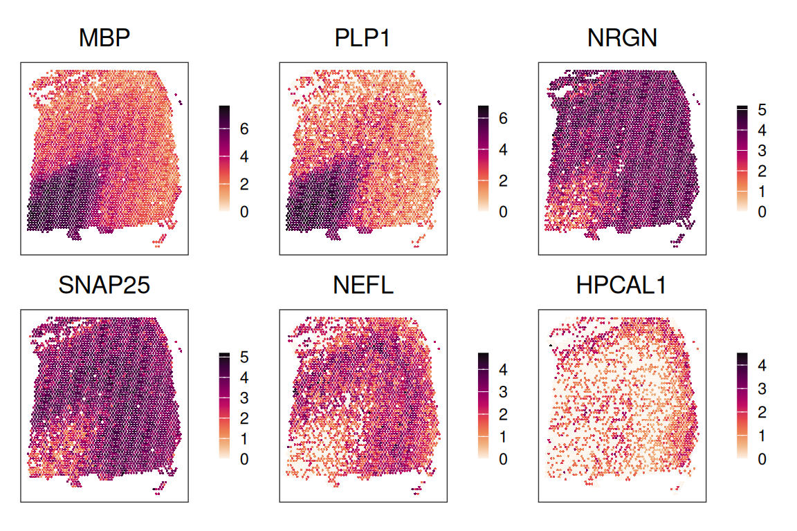

11.8 Appendix

Save data

Save data object for re-use within later chapters.

Code

colLabels(spe) <- spe$BayesSpace
saveRDS(spe, "seq-spe_cl.rds")

References

Bhuva, Dharmesh D., Chin Wee Tan, Agus Salim, Claire Marceaux, Marie A. Pickering, Jinjin Chen, Malvika Kharbanda, et al. 2024. “Library Size Confounds Biology in Spatial Transcriptomics Data.” Genome Biology 25 (99). https://doi.org/10.1186/s13059-024-03241-7.

Maynard, Kristen R., Leonardo Collado-Torres, Lukas M. Weber, Cedric Uytingco, Brianna K. Barry, Stephen R. Williams, Joseph L. Catallini II, et al. 2021. “Transcriptome-Scale Spatial Gene Expression in the Human Dorsolateral Prefrontal Cortex.” Nature Neuroscience 24: 425–36. https://doi.org/10.1038/s41593-020-00787-0.

Salim, Agus, Dharmesh D. Bhuva, Carissa Chen, Chin Wee Tan, Pengyi Yang, Melissa J. Davis, and Jean Y. H. Yang. 2025. “SpaNorm: Spatially-Aware Normalization for Spatial Transcriptomics Data.” Genome Biology 26 (109). https://doi.org/10.1186/s13059-025-03565-y.

Zhao, Edward, Matthew R. Stone, Xing Ren, Jamie Guenthoer, Kimberly S. Smythe, Thomas Pulliam, Stephen R. Williams, et al. 2021. “Spatial Transcriptomics at Subspot Resolution with BayesSpace.” Nature Biotechnology 39: 1375–84. https://doi.org/10.1038/s41587-021-00935-2.