Chapter 1 Correcting batch effects
1.1 Motivation
Large single-cell RNA sequencing (scRNA-seq) projects usually need to generate data across multiple batches due to logistical constraints. However, the processing of different batches is often subject to uncontrollable differences, e.g., changes in operator, differences in reagent quality. This results in systematic differences in the observed expression in cells from different batches, which we refer to as “batch effects”. Batch effects are problematic as they can be major drivers of heterogeneity in the data, masking the relevant biological differences and complicating interpretation of the results.
Computational removal of batch-to-batch variation allows us to combine data across multiple batches for a consolidated downstream analysis. However, existing methods based on linear models (Ritchie et al. 2015; Leek et al. 2012) assume that the composition of cell populations are either known or the same across batches. To overcome these limitations, bespoke methods have been developed for batch correction of single-cell data (Haghverdi et al. 2018; Butler et al. 2018; Lin et al. 2019) that do not require a priori knowledge about the composition of the population. This allows them to be used in workflows for exploratory analyses of scRNA-seq data where such knowledge is usually unavailable.
1.2 Quick start
To demonstrate, we will use two separate 10X Genomics PBMC datasets generated in two different batches. Each dataset was obtained from the TENxPBMCData package and separately subjected to basic processing steps such as quality control and normalization. As a general rule, these upstream processing steps should be done within each batch where possible. For example, outlier-based QC on the cells is more effective when performed within a batch (Advanced Section 1.4), and we can more effectively model the mean-variance relationship on each batch separately (Basic Section 3.4).
#--- loading ---#
library(TENxPBMCData)
all.sce <- list(
    pbmc3k=TENxPBMCData('pbmc3k'),
    pbmc4k=TENxPBMCData('pbmc4k'),
    pbmc8k=TENxPBMCData('pbmc8k')
)

#--- quality-control ---#
library(scater)
stats <- high.mito <- list()
for (n in names(all.sce)) {
    current <- all.sce[[n]]
    is.mito <- grep("MT", rowData(current)$Symbol_TENx)
    stats[[n]] <- perCellQCMetrics(current, subsets=list(Mito=is.mito))
    high.mito[[n]] <- isOutlier(stats[[n]]$subsets_Mito_percent, type="higher")
    all.sce[[n]] <- current[,!high.mito[[n]]]
}

#--- normalization ---#
all.sce <- lapply(all.sce, logNormCounts)

#--- variance-modelling ---#
library(scran)
all.dec <- lapply(all.sce, modelGeneVar)
all.hvgs <- lapply(all.dec, getTopHVGs, prop=0.1)

#--- dimensionality-reduction ---#
library(BiocSingular)
set.seed(10000)
all.sce <- mapply(FUN=runPCA, x=all.sce, subset_row=all.hvgs,
    MoreArgs=list(ncomponents=25, BSPARAM=RandomParam()),
    SIMPLIFY=FALSE)

set.seed(100000)
all.sce <- lapply(all.sce, runTSNE, dimred="PCA")

set.seed(1000000)
all.sce <- lapply(all.sce, runUMAP, dimred="PCA")

#--- clustering ---#
for (n in names(all.sce)) {
    g <- buildSNNGraph(all.sce[[n]], k=10, use.dimred='PCA')
    clust <- igraph::cluster_walktrap(g)$membership
    colLabels(all.sce[[n]])  <- factor(clust)
}## class: SingleCellExperiment
## dim: 32738 2609
## metadata(0):
## assays(2): counts logcounts
## rownames(32738): ENSG00000243485 ENSG00000237613 ... ENSG00000215616
## ENSG00000215611
## rowData names(3): ENSEMBL_ID Symbol_TENx Symbol
## colnames: NULL
## colData names(13): Sample Barcode ... sizeFactor label
## reducedDimNames(3): PCA TSNE UMAP
## mainExpName: NULL
## altExpNames(0):## class: SingleCellExperiment
## dim: 33694 4182
## metadata(0):
## assays(2): counts logcounts
## rownames(33694): ENSG00000243485 ENSG00000237613 ... ENSG00000277475
## ENSG00000268674
## rowData names(3): ENSEMBL_ID Symbol_TENx Symbol
## colnames: NULL
## colData names(13): Sample Barcode ... sizeFactor label
## reducedDimNames(3): PCA TSNE UMAP
## mainExpName: NULL
## altExpNames(0):We then use the quickCorrect() function from the batchelor package to compute corrected values across the two objects.
This performs all the steps to set up the data for correction (Section 1.3),
followed by MNN correction to actually perform the correction itself (Section 1.6).
Algernatively, we could use one of the other correction algorithms described in this chapter by modifying PARAM= appropriately.
library(batchelor)
quick.corrected <- quickCorrect(pbmc3k, pbmc4k,
   precomputed=list(dec3k, dec4k),
   PARAM=FastMnnParam(BSPARAM=BiocSingular::RandomParam()))

quick.sce <- quick.corrected$corrected
quick.sce
## class: SingleCellExperiment
## dim: 31232 6791
## metadata(2): merge.info pca.info
## assays(1): reconstructed
## rownames(31232): ENSG00000243485 ENSG00000237613 ... ENSG00000198695
## ENSG00000198727
## rowData names(1): rotation
## colnames: NULL
## colData names(1): batch
## reducedDimNames(1): corrected
## mainExpName: NULL
## altExpNames(0):This yields low-dimensional corrected values for use in downstream analyses (Figure 1.1).
library(scater)
set.seed(00101010)
quick.sce <- runTSNE(quick.sce, dimred="corrected")
quick.sce$batch <- factor(quick.sce$batch)
plotTSNE(quick.sce, colour_by="batch")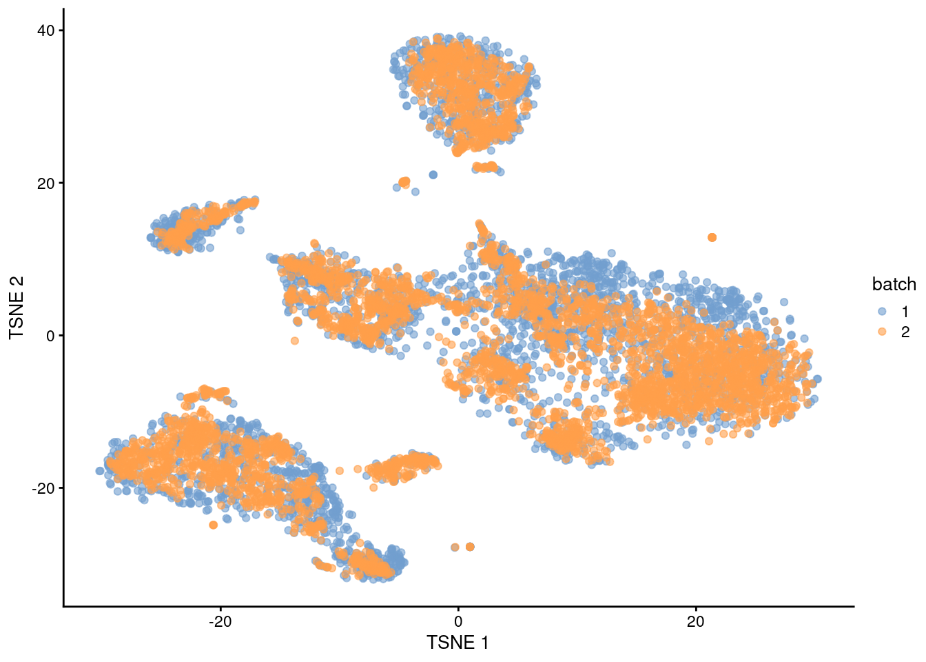
Figure 1.1: \(t\)-SNE plot of the PBMC datasets after MNN correction with quickCorrect(). Each point is a cell that is colored according to its batch of origin.
1.3 Explaining the data preparation
The quickCorrect() function wraps a number of steps that are required to prepare the data for batch correction.
The first and most obvious is to subset all batches to the common “universe” of features.
In this case, it is straightforward as both batches use Ensembl gene annotation;
more difficult integrations will require some mapping of identifiers using packages like org.Mm.eg.db.
## [1] 31232# Subsetting the SingleCellExperiment object.
pbmc3k <- pbmc3k[universe,]
pbmc4k <- pbmc4k[universe,]
# Also subsetting the variance modelling results, for convenience.
dec3k <- dec3k[universe,]
dec4k <- dec4k[universe,]The second step is to rescale each batch to adjust for differences in sequencing depth between batches.
The multiBatchNorm() function recomputes log-normalized expression values after adjusting the size factors for systematic differences in coverage between SingleCellExperiment objects.
(Size factors only remove biases between cells within a single batch.)
This improves the quality of the correction by removing one aspect of the technical differences between batches.
Finally, we perform feature selection by averaging the variance components across all batches with the combineVar() function.
We compute the average as it is responsive to batch-specific HVGs while still preserving the within-batch ranking of genes.
This allows us to use the same strategies described in Basic Section 3.5 to select genes of interest.
In contrast, approaches based on taking the intersection or union of HVGs across batches become increasingly conservative or liberal, respectively, with an increasing number of batches.
library(scran)
combined.dec <- combineVar(dec3k, dec4k)
chosen.hvgs <- combined.dec$bio > 0
sum(chosen.hvgs)
## [1] 13431When integrating datasets of variable composition, it is generally safer to err on the side of including more HVGs than are used in a single dataset analysis, to ensure that markers are retained for any dataset-specific subpopulations that might be present.
For a top \(X\) selection, this means using a larger \(X\) (e.g., quickCorrect() defaults to 5000), or in this case, we simply take all genes above the trend.
That said, many of the signal-to-noise considerations described in Basic Section 3.5 still apply here, so some experimentation may be necessary for best results.
1.4 No correction
Before we actually perform any correction, it is worth examining whether there is any batch effect in this dataset.
We combine the two SingleCellExperiments and perform a PCA on the log-expression values for our selected subset of HVGs.
In this example, our datasets are file-backed and so we instruct runPCA() to use randomized PCA for greater efficiency -
see Advanced Section 14.2.2 for more details - though the default IRLBA will suffice for more common in-memory representations.
# Synchronizing the metadata for cbind()ing.
# TODO: replace with combineCols when that comes out.
rowData(pbmc3k) <- rowData(pbmc4k)
pbmc3k$batch <- "3k"
pbmc4k$batch <- "4k"
uncorrected <- cbind(pbmc3k, pbmc4k)

# Using RandomParam() as it is more efficient for file-backed matrices.
library(scater)
set.seed(0010101010)
uncorrected <- runPCA(uncorrected, subset_row=chosen.hvgs,
    BSPARAM=BiocSingular::RandomParam())
We use graph-based clustering on the components to obtain a summary of the population structure. As our two PBMC populations should be replicates, each cluster should ideally consist of cells from both batches. However, we instead see clusters that are comprised of cells from a single batch. This indicates that cells of the same type are artificially separated due to technical differences between batches.
library(scran)
snn.gr <- buildSNNGraph(uncorrected, use.dimred="PCA")
clusters <- igraph::cluster_walktrap(snn.gr)$membership
tab <- table(Cluster=clusters, Batch=uncorrected$batch)
tab
## Batch
## Cluster 3k 4k
## 1 1 781
## 2 0 1309
## 3 0 535
## 4 14 51
## 5 0 605
## 6 489 0
## 7 0 184
## 8 1272 0
## 9 0 414
## 10 151 0
## 11 0 50
## 12 155 0
## 13 0 65
## 14 0 61
## 15 0 88
## 16 30 0
## 17 339 0
## 18 145 0
## 19 11 3
## 20 2 36This is supported by the \(t\)-SNE visualization (Figure 1.2). where the strong separation between cells from different batches is consistent with the clustering results.
set.seed(1111001)
uncorrected <- runTSNE(uncorrected, dimred="PCA")
plotTSNE(uncorrected, colour_by="batch")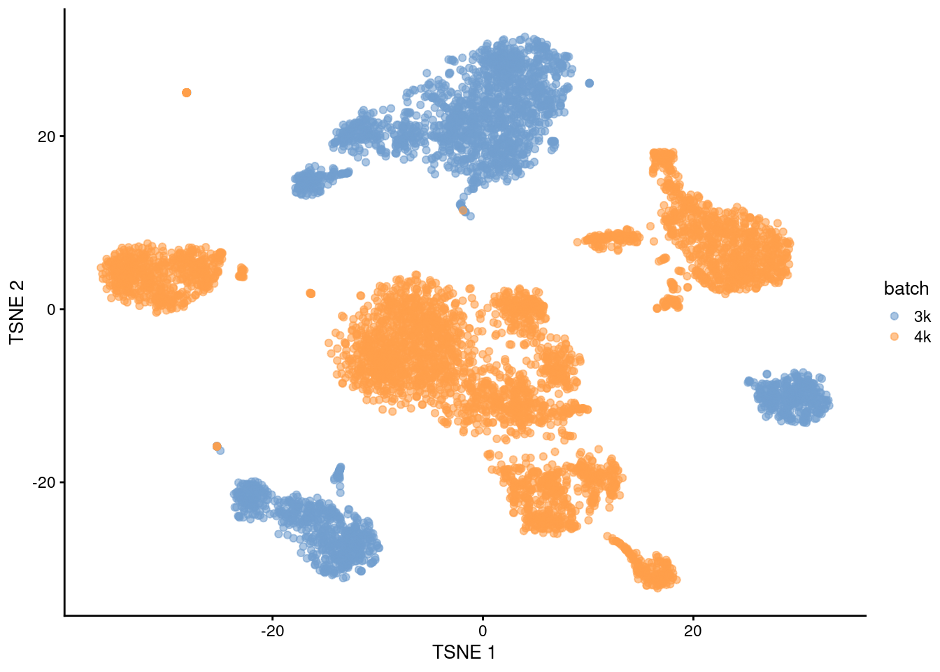
Figure 1.2: \(t\)-SNE plot of the PBMC datasets without any batch correction. Each point is a cell that is colored according to its batch of origin.
Of course, the other explanation for batch-specific clusters is that there are cell types that are unique to each batch. The degree of intermingling of cells from different batches is not an effective diagnostic when the batches involved might actually contain unique cell subpopulations (which is not a consideration in the PBMC dataset, but the same cannot be said in general). If a cluster only contains cells from a single batch, one can always debate whether that is caused by a failure of the correction method or if there is truly a batch-specific subpopulation. For example, do batch-specific metabolic or differentiation states represent distinct subpopulations? Or should they be merged together? We will not attempt to answer this here, only noting that each batch correction algorithm will make different (and possibly inappropriate) decisions on what constitutes “shared” and “unique” populations.
1.5 Linear regression
1.5.1 By rescaling the counts
Batch effects in bulk RNA sequencing studies are commonly removed with linear regression.
This involves fitting a linear model to each gene’s expression profile, setting the undesirable batch term to zero and recomputing the observations sans the batch effect, yielding a set of corrected expression values for downstream analyses.
Linear modelling is the basis of the removeBatchEffect() function from the limma package (Ritchie et al. 2015) as well the comBat() function from the sva package (Leek et al. 2012).
To use this approach in a scRNA-seq context, we assume that the composition of cell subpopulations is the same across batches. We also assume that the batch effect is additive, i.e., any batch-induced fold-change in expression is the same across different cell subpopulations for any given gene. These are strong assumptions as batches derived from different individuals will naturally exhibit variation in cell type abundances and expression. Nonetheless, they may be acceptable when dealing with batches that are technical replicates generated from the same population of cells. (In fact, when its assumptions hold, linear regression is the most statistically efficient as it uses information from all cells to compute the common batch vector.) Linear modelling can also accommodate situations where the composition is known a priori by including the cell type as a factor in the linear model, but this situation is even less common.
We use the rescaleBatches() function from the batchelor package to remove the batch effect.
This is roughly equivalent to applying a linear regression to the log-expression values per gene, with some adjustments to improve performance and efficiency.
For each gene, the mean expression in each batch is scaled down until it is equal to the lowest mean across all batches.
We deliberately choose to scale all expression values down as this mitigates differences in variance when batches lie at different positions on the mean-variance trend.
(Specifically, the shrinkage effect of the pseudo-count is greater for smaller counts, suppressing any differences in variance across batches.)
An additional feature of rescaleBatches() is that it will preserve sparsity in the input matrix for greater efficiency, whereas other methods like removeBatchEffect() will always return a dense matrix.
## class: SingleCellExperiment
## dim: 31232 6791
## metadata(0):
## assays(1): corrected
## rownames(31232): ENSG00000243485 ENSG00000237613 ... ENSG00000198695
##   ENSG00000198727
## rowData names(0):
## colnames: NULL
## colData names(1): batch
## reducedDimNames(0):
## mainExpName: NULL
## altExpNames(0):
The corrected expression values can be used in place of the "logcounts" assay in PCA and clustering (see Chapter 3).
After clustering, we observe that most clusters consist of mixtures of cells from the two replicate batches, consistent with the removal of the batch effect.
This conclusion is supported by the apparent mixing of cells from different batches in Figure 1.3.
However, at least one batch-specific cluster is still present, indicating that the correction is not entirely complete.
This is attributable to violation of one of the aforementioned assumptions, even in this simple case involving replicated batches.
# To ensure reproducibility of the randomized PCA.
set.seed(1010101010)
rescaled <- runPCA(rescaled, subset_row=chosen.hvgs,
    exprs_values="corrected",
    BSPARAM=BiocSingular::RandomParam())

snn.gr <- buildSNNGraph(rescaled, use.dimred="PCA")
clusters.resc <- igraph::cluster_walktrap(snn.gr)$membership
tab.resc <- table(Cluster=clusters.resc, Batch=rescaled$batch)
tab.resc
## Batch
## Cluster 1 2
## 1 278 525
## 2 16 23
## 3 337 606
## 4 43 748
## 5 604 529
## 6 22 71
## 7 188 48
## 8 25 49
## 9 263 0
## 10 123 135
## 11 16 85
## 12 11 57
## 13 116 6
## 14 455 1035
## 15 6 31
## 16 89 187
## 17 3 36
## 18 3 8
## 19 11 3rescaled <- runTSNE(rescaled, dimred="PCA")
rescaled$batch <- factor(rescaled$batch)
plotTSNE(rescaled, colour_by="batch")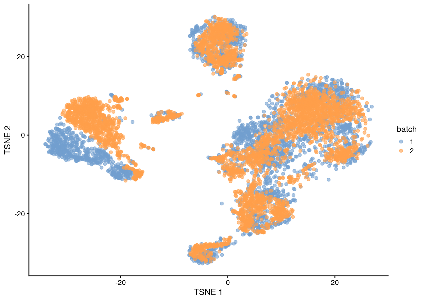
Figure 1.3: \(t\)-SNE plot of the PBMC datasets after correction with rescaleBatches(). Each point represents a cell and is colored according to the batch of origin.
1.5.2 By fitting a linear model
Alternatively, we could use the regressBatches() function to perform a more conventional linear regression for batch correction.
This is subject to the same assumptions as described above for rescaleBatches(), though it has the additional disadvantage of discarding sparsity in the matrix of residuals.
To avoid this, we avoid explicit calculation of the residuals during matrix multiplication (see ?ResidualMatrix for details), allowing us to perform an approximate PCA more efficiently.
Advanced users can set design= and specify which coefficients to retain in the output matrix, reminiscent of limma’s removeBatchEffect() function.
set.seed(10001)
residuals <- regressBatches(pbmc3k, pbmc4k, d=50,
    subset.row=chosen.hvgs, correct.all=TRUE,
    BSPARAM=BiocSingular::RandomParam())
We set d=50 to instruct regressBatches() to automatically perform a PCA for us.
The PCs derived from the residuals can then be used in clustering and further dimensionality reduction, as demonstrated in Figure 1.4.
snn.gr <- buildSNNGraph(residuals, use.dimred="corrected")
clusters.resid <- igraph::cluster_walktrap(snn.gr)$membership
tab.resid <- table(Cluster=clusters.resid, Batch=residuals$batch)
tab.resid
## Batch
## Cluster 1 2
## 1 478 2
## 2 142 179
## 3 22 41
## 4 298 566
## 5 340 606
## 6 0 138
## 7 404 376
## 8 145 91
## 9 2 636
## 10 22 73
## 11 6 51
## 12 629 1110
## 13 3 36
## 14 91 211
## 15 12 55
## 16 4 8
## 17 11 3residuals <- runTSNE(residuals, dimred="corrected")
residuals$batch <- factor(residuals$batch)
plotTSNE(residuals, colour_by="batch")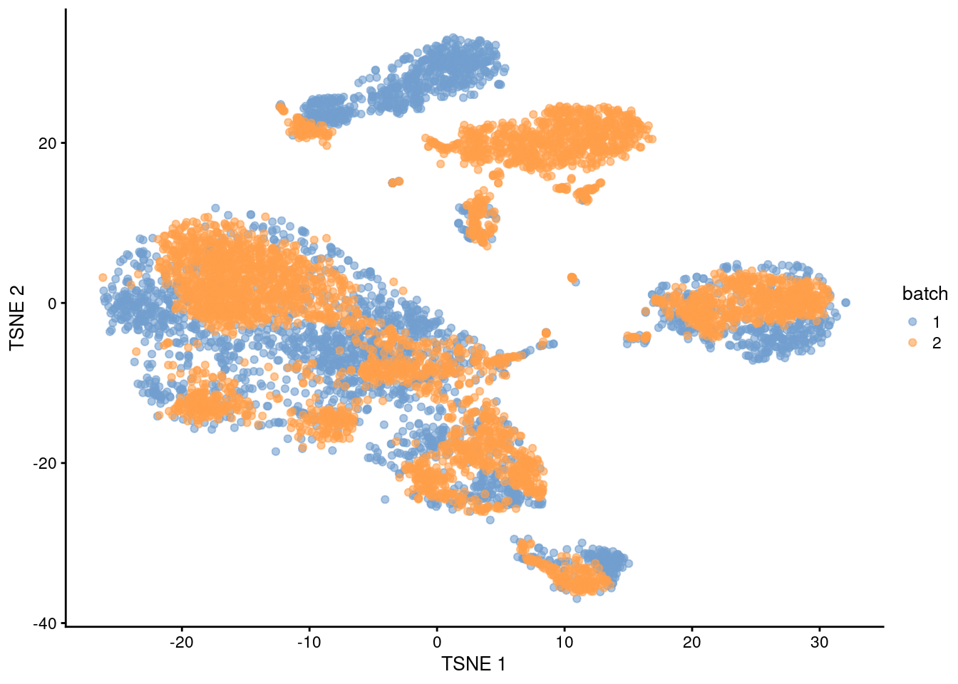
Figure 1.4: \(t\)-SNE plot of the PBMC datasets after correction with regressBatches(). Each point represents a cell and is colored according to the batch of origin.
1.6 MNN correction
Consider a cell \(a\) in batch \(A\), and identify the cells in batch \(B\) that are nearest neighbors to \(a\) in the expression space defined by the selected features. Repeat this for a cell \(b\) in batch \(B\), identifying its nearest neighbors in \(A\). Mutual nearest neighbors are pairs of cells from different batches that belong in each other’s set of nearest neighbors. The reasoning is that MNN pairs represent cells from the same biological state prior to the application of a batch effect - see Haghverdi et al. (2018) for full theoretical details. Thus, the difference between cells in MNN pairs can be used as an estimate of the batch effect, the subtraction of which yields batch-corrected values.
Compared to linear regression, MNN correction does not assume that the population composition is the same or known beforehand. This is because it learns the shared population structure via identification of MNN pairs and uses this information to obtain an appropriate estimate of the batch effect. Instead, the key assumption of MNN-based approaches is that the batch effect is orthogonal to the biology in high-dimensional expression space. Violations reduce the effectiveness and accuracy of the correction, with the most common case arising from variations in the direction of the batch effect between clusters. Nonetheless, the assumption is usually reasonable as a random vector is very likely to be orthogonal in high-dimensional space.
The batchelor package provides an implementation of the MNN approach via the fastMNN() function.
(Unlike the MNN method originally described by Haghverdi et al. (2018), the fastMNN() function performs PCA to reduce the dimensions beforehand and speed up the downstream neighbor detection steps.)
We apply it to our two PBMC batches to remove the batch effect across the highly variable genes in chosen.hvgs.
To reduce computational work and technical noise, all cells in all batches are projected into the low-dimensional space defined by the top d principal components.
Identification of MNNs and calculation of correction vectors are then performed in this low-dimensional space.
# Again, using randomized SVD here, as this is faster than IRLBA for
# file-backed matrices. We set deferred=TRUE for greater speed.
set.seed(1000101001)
mnn.out <- fastMNN(pbmc3k, pbmc4k, d=50, k=20, subset.row=chosen.hvgs,
    BSPARAM=BiocSingular::RandomParam(deferred=TRUE))
mnn.out
## class: SingleCellExperiment
## dim: 13431 6791
## metadata(2): merge.info pca.info
## assays(1): reconstructed
## rownames(13431): ENSG00000239945 ENSG00000228463 ... ENSG00000198695
## ENSG00000198727
## rowData names(1): rotation
## colnames: NULL
## colData names(1): batch
## reducedDimNames(1): corrected
## mainExpName: NULL
## altExpNames(0):The function returns a SingleCellExperiment object containing corrected values for downstream analyses like clustering or visualization.
Each column of mnn.out corresponds to a cell in one of the batches, while each row corresponds to an input gene in chosen.hvgs.
The batch field in the column metadata contains a vector specifying the batch of origin of each cell.
## [1] 1 1 1 1 1 1The corrected matrix in the reducedDims() contains the low-dimensional corrected coordinates for all cells, which we will use in place of the PCs in our downstream analyses.
## [1] 6791 50A reconstructed matrix in the assays() contains the corrected expression values for each gene in each cell, obtained by projecting the low-dimensional coordinates in corrected back into gene expression space.
We do not recommend using this for anything other than visualization (Chapter 3).
## <13431 x 6791> matrix of class LowRankMatrix and type "double":
##                       [,1]       [,2]       [,3] ...    [,6790]    [,6791]
## ENSG00000239945 -2.522e-06 -1.851e-06 -1.199e-05   .  1.832e-06 -3.641e-06
## ENSG00000228463 -6.627e-04 -6.724e-04 -4.820e-04   . -8.531e-04 -3.999e-04
## ENSG00000237094 -8.077e-05 -8.038e-05 -9.631e-05   .  7.261e-06 -4.094e-05
## ENSG00000229905  3.838e-06  6.180e-06  5.432e-06   .  8.534e-06  3.485e-06
## ENSG00000237491 -4.527e-04 -3.178e-04 -1.510e-04   . -3.491e-04 -2.082e-04
##             ...          .          .          .   .          .          .
## ENSG00000198840 -0.0296508 -0.0340101 -0.0502385   . -0.0362884 -0.0183084
## ENSG00000212907 -0.0041681 -0.0056570 -0.0106420   . -0.0083837  0.0005996
## ENSG00000198886  0.0145358  0.0200517 -0.0307131   . -0.0109254 -0.0070064
## ENSG00000198695  0.0014427  0.0013490  0.0001493   . -0.0009826 -0.0022712
## ENSG00000198727  0.0152570  0.0106167 -0.0256450   . -0.0227962 -0.0022898
The most relevant parameter for tuning fastMNN() is k, which specifies the number of nearest neighbors to consider when defining MNN pairs.
This can be interpreted as the minimum anticipated frequency of any shared cell type or state in each batch.
Increasing k will generally result in more aggressive merging as the algorithm is more generous in matching subpopulations across batches.
It can occasionally be desirable to increase k if one clearly sees that the same cell types are not being adequately merged across batches.
We cluster on the low-dimensional corrected coordinates to obtain a partitioning of the cells that serves as a proxy for the population structure. If the batch effect is successfully corrected, clusters corresponding to shared cell types or states should contain cells from multiple batches. We see that all clusters contain contributions from each batch after correction, consistent with our expectation that the two batches are replicates of each other.
library(scran)
snn.gr <- buildSNNGraph(mnn.out, use.dimred="corrected")
clusters.mnn <- igraph::cluster_walktrap(snn.gr)$membership
tab.mnn <- table(Cluster=clusters.mnn, Batch=mnn.out$batch)
tab.mnn
## Batch
## Cluster 1 2
## 1 337 606
## 2 289 542
## 3 152 181
## 4 12 4
## 5 517 467
## 6 17 19
## 7 313 661
## 8 162 118
## 9 11 56
## 10 547 1083
## 11 17 59
## 12 16 58
## 13 144 93
## 14 67 191
## 15 4 36
## 16 4 8We can also visualize the corrected coordinates using a \(t\)-SNE plot (Figure 1.5). The presence of visual clusters containing cells from both batches provides a comforting illusion that the correction was successful.
library(scater)
set.seed(0010101010)
mnn.out <- runTSNE(mnn.out, dimred="corrected")

mnn.out$batch <- factor(mnn.out$batch)
plotTSNE(mnn.out, colour_by="batch")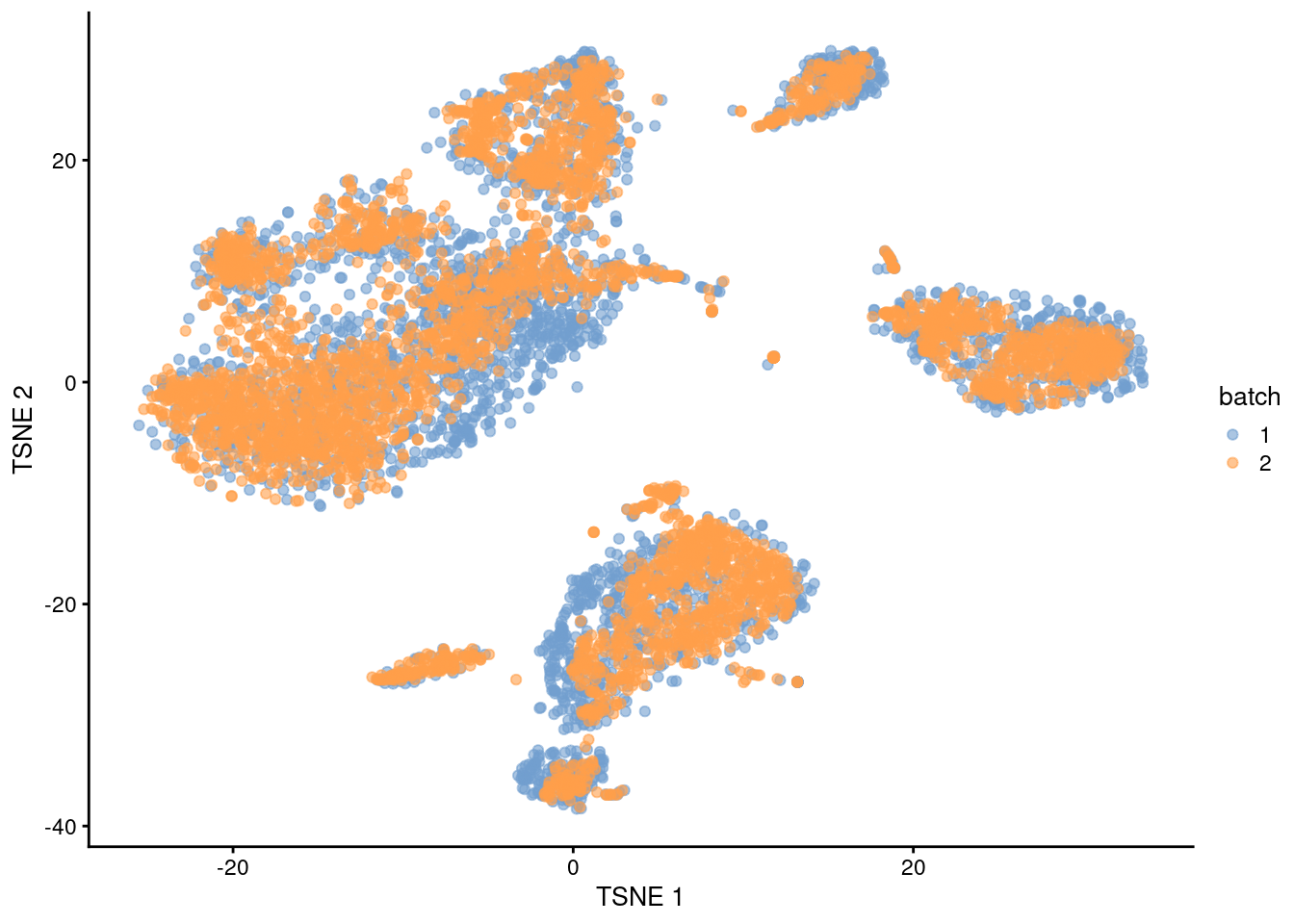
Figure 1.5: \(t\)-SNE plot of the PBMC datasets after MNN correction with fastMNN(). Each point is a cell that is colored according to its batch of origin.
See also Chapter 8 for a case study using MNN correction on a series of human pancreas datasets.
1.7 Further options
All of the batchelor functions can operate on a single SingleCellExperiment containing data from all batches.
For example, if we were to recycle the uncorrected object from Section 1.4, we could apply MNN correction without splitting the object into multiple parts.
set.seed(10000)
single.correct <- fastMNN(uncorrected, batch=uncorrected$batch,
    subset.row=chosen.hvgs, BSPARAM=BiocSingular::RandomParam())
single.correct
## class: SingleCellExperiment
## dim: 13431 6791
## metadata(2): merge.info pca.info
## assays(1): reconstructed
## rownames(13431): ENSG00000239945 ENSG00000228463 ... ENSG00000198695
## ENSG00000198727
## rowData names(1): rotation
## colnames: NULL
## colData names(1): batch
## reducedDimNames(1): corrected
## mainExpName: NULL
## altExpNames(0):It is similarly straightforward to simultaneously perform correction across >2 batches,
either by having multiple levels in batch= or by providing more SingleCellExperiment objects (or even raw matrices of expression values).
This is demonstrated below for MNN correction with an additional PBMC dataset (Figure 1.6).
pbmc8k <- all.sce$pbmc8k
dec8k <- all.dec$pbmc8k

quick.corrected2 <- quickCorrect(`3k`=pbmc3k, `4k`=pbmc4k, `8k`=pbmc8k,
   precomputed=list(dec3k, dec4k, dec8k),
   PARAM=FastMnnParam(BSPARAM=BiocSingular::RandomParam(), auto.merge=TRUE))

quick.sce2 <- quick.corrected2$corrected

set.seed(00101010)
quick.sce2 <- runTSNE(quick.sce2, dimred="corrected")
plotTSNE(quick.sce2, colour_by="batch")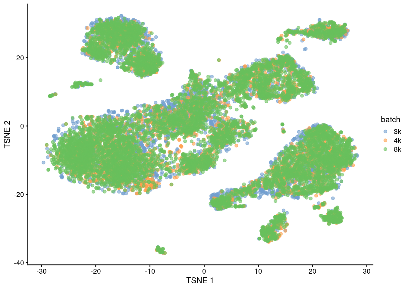
Figure 1.6: Yet another \(t\)-SNE plot of the PBMC datasets after MNN correction. Each point is a cell that is colored according to its batch of origin.
In the specific case of MNN correction, we can also set auto.merge=TRUE to allow it to choose the “best” order in which to perform the merges.
This is slower but can occasionally be useful when the batches involved have very different cell type compositions.
For example, if one batch contained only B cells, another batch contained only T cells and a third batch contained B and T cells,
it would be unwise to try to merge the first two batches together as the wrong MNN pairs would be identified.
With auto.merge=TRUE, the function would automatically recognize that the third batch should be used as the reference to which the others should be merged.
Session Info
R version 4.1.0 beta (2021-05-03 r80259)
Platform: x86_64-pc-linux-gnu (64-bit)
Running under: Ubuntu 20.04.2 LTS

Matrix products: default
BLAS:   /home/biocbuild/bbs-3.14-bioc/R/lib/libRblas.so
LAPACK: /home/biocbuild/bbs-3.14-bioc/R/lib/libRlapack.so

locale:
 [1] LC_CTYPE=en_US.UTF-8       LC_NUMERIC=C
 [3] LC_TIME=en_GB              LC_COLLATE=C
 [5] LC_MONETARY=en_US.UTF-8    LC_MESSAGES=en_US.UTF-8
 [7] LC_PAPER=en_US.UTF-8       LC_NAME=C
 [9] LC_ADDRESS=C               LC_TELEPHONE=C
[11] LC_MEASUREMENT=en_US.UTF-8 LC_IDENTIFICATION=C

attached base packages:
[1] parallel  stats4    stats     graphics  grDevices utils     datasets
[8] methods   base

other attached packages:
 [1] scran_1.21.1                scater_1.21.0
 [3] ggplot2_3.3.3               scuttle_1.3.0
 [5] batchelor_1.9.0             SingleCellExperiment_1.15.1
 [7] SummarizedExperiment_1.23.0 Biobase_2.53.0
 [9] GenomicRanges_1.45.0        GenomeInfoDb_1.29.0
[11] HDF5Array_1.21.0            rhdf5_2.37.0
[13] DelayedArray_0.19.0         IRanges_2.27.0
[15] S4Vectors_0.31.0            MatrixGenerics_1.5.0
[17] matrixStats_0.58.0          BiocGenerics_0.39.0
[19] Matrix_1.3-3                BiocStyle_2.21.0
[21] rebook_1.3.0

loaded via a namespace (and not attached):
 [1] bitops_1.0-7              filelock_1.0.2
 [3] tools_4.1.0               bslib_0.2.5.1
 [5] utf8_1.2.1                R6_2.5.0
 [7] irlba_2.3.3               ResidualMatrix_1.3.0
 [9] vipor_0.4.5               DBI_1.1.1
[11] colorspace_2.0-1          rhdf5filters_1.5.0
[13] withr_2.4.2               gridExtra_2.3
[15] tidyselect_1.1.1          compiler_4.1.0
[17] graph_1.71.0              BiocNeighbors_1.11.0
[19] labeling_0.4.2            bookdown_0.22
[21] sass_0.4.0                scales_1.1.1
[23] stringr_1.4.0             digest_0.6.27
[25] rmarkdown_2.8             XVector_0.33.0
[27] pkgconfig_2.0.3           htmltools_0.5.1.1
[29] sparseMatrixStats_1.5.0   highr_0.9
[31] limma_3.49.0              rlang_0.4.11
[33] DelayedMatrixStats_1.15.0 farver_2.1.0
[35] generics_0.1.0            jquerylib_0.1.4
[37] jsonlite_1.7.2            BiocParallel_1.27.0
[39] dplyr_1.0.6               RCurl_1.98-1.3
[41] magrittr_2.0.1            BiocSingular_1.9.0
[43] GenomeInfoDbData_1.2.6    ggbeeswarm_0.6.0
[45] Rcpp_1.0.6                munsell_0.5.0
[47] Rhdf5lib_1.15.0           fansi_0.4.2
[49] viridis_0.6.1             lifecycle_1.0.0
[51] stringi_1.6.2             yaml_2.2.1
[53] edgeR_3.35.0              zlibbioc_1.39.0
[55] Rtsne_0.15                grid_4.1.0
[57] dqrng_0.3.0               crayon_1.4.1
[59] dir.expiry_1.1.0          lattice_0.20-44
[61] cowplot_1.1.1             beachmat_2.9.0
[63] locfit_1.5-9.4            CodeDepends_0.6.5
[65] metapod_1.1.0             knitr_1.33
[67] pillar_1.6.1              igraph_1.2.6
[69] codetools_0.2-18          ScaledMatrix_1.1.0
[71] XML_3.99-0.6              glue_1.4.2
[73] evaluate_0.14             BiocManager_1.30.15
[75] vctrs_0.3.8               purrr_0.3.4
[77] gtable_0.3.0              assertthat_0.2.1
[79] xfun_0.23                 rsvd_1.0.5
[81] viridisLite_0.4.0         tibble_3.1.2
[83] beeswarm_0.3.1            cluster_2.1.2
[85] bluster_1.3.0             statmod_1.4.36
[87] ellipsis_0.3.2
References
Butler, A., P. Hoffman, P. Smibert, E. Papalexi, and R. Satija. 2018. “Integrating single-cell transcriptomic data across different conditions, technologies, and species.” Nat. Biotechnol. 36 (5): 411–20.
Haghverdi, L., A. T. L. Lun, M. D. Morgan, and J. C. Marioni. 2018. “Batch effects in single-cell RNA-sequencing data are corrected by matching mutual nearest neighbors.” Nat. Biotechnol. 36 (5): 421–27.
Leek, J. T., W. E. Johnson, H. S. Parker, A. E. Jaffe, and J. D. Storey. 2012. “The sva package for removing batch effects and other unwanted variation in high-throughput experiments.” Bioinformatics 28 (6): 882–83.
Lin, Y., S. Ghazanfar, K. Y. X. Wang, J. A. Gagnon-Bartsch, K. K. Lo, X. Su, Z. G. Han, et al. 2019. “scMerge leverages factor analysis, stable expression, and pseudoreplication to merge multiple single-cell RNA-seq datasets.” Proc. Natl. Acad. Sci. U.S.A. 116 (20): 9775–84.
Ritchie, M. E., B. Phipson, D. Wu, Y. Hu, C. W. Law, W. Shi, and G. K. Smyth. 2015. “limma powers differential expression analyses for RNA-sequencing and microarray studies.” Nucleic Acids Res. 43 (7): e47.