Chapter 5 Problems with ambient RNA
5.1 Background
Ambient contamination is a phenomenon that is generally most pronounced in massively multiplexed scRNA-seq protocols. Briefly, extracellular RNA (most commonly released upon cell lysis) is captured along with each cell in its reaction chamber, contributing counts to genes that are not otherwise expressed in that cell (see Advanced Section 7.2). Differences in the ambient profile across samples are not uncommon when dealing with strong experimental perturbations where strong expression of a gene in a condition-specific cell type can “bleed over” into all other cell types in the same sample. This is problematic for DE analyses between conditions, as DEGs detected for a particular cell type may be driven by differences in the ambient profiles rather than any intrinsic change in gene regulation.
To illustrate, we consider the Tal1-knockout (KO) chimera data from Pijuan-Sala et al. (2019). This is very similar to the WT chimera dataset we previously examined, only differing in that the Tal1 gene was knocked out in the injected cells. Tal1 is a transcription factor that has known roles in erythroid differentiation; the aim of the experiment was to determine if blocking of the erythroid lineage diverted cells to other developmental fates. (To cut a long story short: yes, it did.)
library(MouseGastrulationData)
sce.tal1 <- Tal1ChimeraData()

library(scuttle)
rownames(sce.tal1) <- uniquifyFeatureNames(
    rowData(sce.tal1)$ENSEMBL,
    rowData(sce.tal1)$SYMBOL
)
sce.tal1
## class: SingleCellExperiment
## dim: 29453 56122
## metadata(0):
## assays(1): counts
## rownames(29453): Xkr4 Gm1992 ... CAAA01147332.1 tomato-td
## rowData names(2): ENSEMBL SYMBOL
## colnames(56122): cell_1 cell_2 ... cell_56121 cell_56122
## colData names(9): cell barcode ... pool sizeFactor
## reducedDimNames(1): pca.corrected
## mainExpName: NULL
## altExpNames(0):We will perform a DE analysis between WT and KO cells labelled as “neural crest”. We observe that the strongest DEGs are the hemoglobins, which are downregulated in the injected cells. This is rather surprising as these cells are distinct from the erythroid lineage and should not express hemoglobins at all. The most sober explanation is that the background samples contain more hemoglobin transcripts in the ambient solution due to leakage from erythrocytes (or their precursors) during sorting and dissociation.
library(scran)
summed.tal1 <- aggregateAcrossCells(sce.tal1,
    ids=DataFrame(sample=sce.tal1$sample,
        label=sce.tal1$celltype.mapped)
)
summed.tal1$block <- summed.tal1$sample %% 2 == 0 # Add blocking factor.

# Subset to our neural crest cells.
summed.neural <- summed.tal1[,summed.tal1$label=="Neural crest"]
summed.neural
## class: SingleCellExperiment
## dim: 29453 4
## metadata(0):
## assays(1): counts
## rownames(29453): Xkr4 Gm1992 ... CAAA01147332.1 tomato-td
## rowData names(2): ENSEMBL SYMBOL
## colnames: NULL
## colData names(13): cell barcode ... ncells block
## reducedDimNames(1): pca.corrected
## mainExpName: NULL
## altExpNames(0):# Standard edgeR analysis, as described in previous chapters.
res.neural <- pseudoBulkDGE(summed.neural,
label=summed.neural$label,
design=~factor(block) + tomato,
coef="tomatoTRUE",
condition=summed.neural$tomato)
summarizeTestsPerLabel(decideTestsPerLabel(res.neural))## -1 0 1 NA
## Neural crest 351 9818 481 18803# Summary of the direction of log-fold changes.
tab.neural <- res.neural[[1]]
tab.neural <- tab.neural[order(tab.neural$PValue),]
head(tab.neural, 10)## DataFrame with 10 rows and 5 columns
## logFC logCPM F PValue FDR
## <numeric> <numeric> <numeric> <numeric> <numeric>
## Xist -7.555686 8.21232 6657.298 0.00000e+00 0.00000e+00
## Hbb-bh1 -8.091042 9.15972 10758.256 0.00000e+00 0.00000e+00
## Hbb-y -8.415622 8.35705 7364.290 0.00000e+00 0.00000e+00
## Hba-x -7.724803 8.53284 7896.457 0.00000e+00 0.00000e+00
## Hba-a1 -8.596706 6.74429 2756.573 0.00000e+00 0.00000e+00
## Hba-a2 -8.866232 5.81300 1517.726 1.72378e-310 3.05972e-307
## Erdr1 1.889536 7.61593 1407.112 2.34678e-289 3.57046e-286
## Cdkn1c -8.864528 4.96097 814.936 8.79979e-173 1.17147e-169
## Uba52 -0.879668 8.38618 424.191 1.86585e-92 2.20792e-89
## Grb10 -1.403427 6.58314 401.353 1.13898e-87 1.21302e-84As an aside, it is worth mentioning that the “replicates” in this study are more technical than biological, so some exaggeration of the significance of the effects is to be expected. Nonetheless, it is a useful dataset to demonstrate some strategies for mitigating issues caused by ambient contamination.
5.2 Filtering out affected DEGs
5.2.1 By estimating ambient contamination
As shown above, the presence of ambient contamination makes it difficult to interpret multi-condition DE analyses.
To mitigate its effects, we need to obtain an estimate of the ambient “expression” profile from the raw count matrix for each sample.
We follow the approach used in emptyDrops() (Lun et al. 2019) and consider all barcodes with total counts below 100 to represent empty droplets.
We then sum the counts for each gene across these barcodes to obtain an expression vector representing the ambient profile for each sample.
library(DropletUtils)
ambient <- vector("list", ncol(summed.neural))

# Looping over all raw (unfiltered) count matrices and
# computing the ambient profile based on its low-count barcodes.
# Turning off rounding, as we know this is count data.
for (s in seq_along(ambient)) {
    raw.tal1 <- Tal1ChimeraData(type="raw", samples=s)[[1]]
    ambient[[s]] <- ambientProfileEmpty(counts(raw.tal1),
        good.turing=FALSE, round=FALSE)
}

# Cleaning up the output for pretty printing.
ambient <- do.call(cbind, ambient)
colnames(ambient) <- seq_len(ncol(ambient))
rownames(ambient) <- uniquifyFeatureNames(
    rowData(raw.tal1)$ENSEMBL,
    rowData(raw.tal1)$SYMBOL
)
head(ambient)
## 1 2 3 4
## Xkr4 1 0 0 0
## Gm1992 0 0 0 0
## Gm37381 1 0 1 0
## Rp1 0 1 0 1
## Sox17 76 76 31 53
## Gm37323 0 0 0 0For each sample, we determine the maximum proportion of the count for each gene that could be attributed to ambient contamination.
This is done by scaling the ambient profile in ambient to obtain a per-gene expected count from ambient contamination, with which we compute the \(p\)-value for observing a count equal to or lower than that in summed.neural.
We perform this for a range of scaling factors and identify the largest factor that yields a \(p\)-value above a given threshold.
The scaled ambient profile represents the upper bound of the contribution to each sample from ambient contamination.
We deliberately use an upper bound so that our next step will aggressively remove any gene that is potentially problematic.
max.ambient <- ambientContribMaximum(counts(summed.neural),
    ambient, mode="proportion")
head(max.ambient)
## [,1] [,2] [,3] [,4]
## Xkr4 NaN NaN NaN NaN
## Gm1992 NaN NaN NaN NaN
## Gm37381 NaN NaN NaN NaN
## Rp1 NaN NaN NaN NaN
## Sox17 0.1775 0.1833 0.468 1
## Gm37323 NaN NaN NaN NaNGenes in which over 10% of the counts are ambient-derived are subsequently discarded from our analysis. For balanced designs, this threshold prevents ambient contribution from biasing the true fold-change by more than 10%, which is a tolerable margin of error for most applications. (Unbalanced designs may warrant the use of a weighted average to account for sample size differences between groups.) This approach yields a slightly smaller list of DEGs without the hemoglobins, which is encouraging as it suggests that any other, less obvious effects of ambient contamination have also been removed.
# Averaging the ambient contribution across samples.
contamination <- rowMeans(max.ambient, na.rm=TRUE)
non.ambient <- contamination <= 0.1
summary(non.ambient)
## Mode FALSE TRUE NA's
## logical 1475 15306 12672okay.genes <- names(non.ambient)[which(non.ambient)]
tab.neural2 <- tab.neural[rownames(tab.neural) %in% okay.genes,]
table(Direction=tab.neural2$logFC > 0, Significant=tab.neural2$FDR <= 0.05)## Significant
## Direction FALSE TRUE
## FALSE 4820 317
## TRUE 4781 452## DataFrame with 10 rows and 5 columns
## logFC logCPM F PValue FDR
## <numeric> <numeric> <numeric> <numeric> <numeric>
## Xist -7.555686 8.21232 6657.298 0.00000e+00 0.00000e+00
## Erdr1 1.889536 7.61593 1407.112 2.34678e-289 3.57046e-286
## Uba52 -0.879668 8.38618 424.191 1.86585e-92 2.20792e-89
## Grb10 -1.403427 6.58314 401.353 1.13898e-87 1.21302e-84
## Gt(ROSA)26Sor 1.481294 5.71617 351.940 2.80072e-77 2.71160e-74
## Fdps 0.981388 7.21805 337.159 3.67655e-74 3.26294e-71
## Mest 0.549349 10.98269 319.697 1.79833e-70 1.47324e-67
## Impact 1.396666 5.71801 314.700 2.05057e-69 1.55990e-66
## H13 -1.481658 5.90902 301.675 1.17372e-66 8.33343e-64
## Msmo1 1.493771 5.43923 301.066 1.57983e-66 1.05158e-63A softer approach is to simply report the average contaminating percentage for each gene in the table of DE statistics.
Readers can then make up their own minds as to whether a particular DEG’s effect is driven by ambient contamination.
Indeed, it is worth remembering that maximumAmbience() will report the maximum possible contamination rather than attempting to estimate the actual level of contamination, and filtering on the former may be too conservative.
This is especially true for cell populations that are contributing to the differences in the ambient pool; in the most extreme case, the reported maximum contamination would be 100% for cell types with an expression profile that is identical to the ambient pool.
tab.neural3 <- tab.neural
tab.neural3$contamination <- contamination[rownames(tab.neural3)]
head(tab.neural3)
## DataFrame with 6 rows and 6 columns
## logFC logCPM F PValue FDR contamination
## <numeric> <numeric> <numeric> <numeric> <numeric> <numeric>
## Xist -7.55569 8.21232 6657.30 0.00000e+00 0.00000e+00 0.0605735
## Hbb-bh1 -8.09104 9.15972 10758.26 0.00000e+00 0.00000e+00 0.9900717
## Hbb-y -8.41562 8.35705 7364.29 0.00000e+00 0.00000e+00 0.9674483
## Hba-x -7.72480 8.53284 7896.46 0.00000e+00 0.00000e+00 0.9945348
## Hba-a1 -8.59671 6.74429 2756.57 0.00000e+00 0.00000e+00 0.8626846
## Hba-a2 -8.86623 5.81300 1517.73 1.72378e-310 3.05972e-307 0.73514035.2.2 With prior knowledge
Another strategy to estimating the ambient proportions involves the use of prior knowledge of mutually exclusive gene expression profiles (Young and Behjati 2018).
In this case, we assume (reasonably) that hemoglobins should not be expressed in neural crest cells and use this to estimate the contamination in each sample.
This is achieved with the controlAmbience() function, which scales the ambient profile so that the hemoglobin coverage is the same as the corresponding sample of summed.neural.
From these profiles, we compute proportions of ambient contamination that are used to mark or filter out affected genes in the same manner as described above.
is.hbb <- grep("^Hb[ab]-", rownames(summed.neural))
ctrl.ambient <- ambientContribNegative(counts(summed.neural), ambient,
    features=is.hbb,  mode="proportion")
head(ctrl.ambient)
## [,1] [,2] [,3] [,4]
## Xkr4 NaN NaN NaN NaN
## Gm1992 NaN NaN NaN NaN
## Gm37381 NaN NaN NaN NaN
## Rp1 NaN NaN NaN NaN
## Sox17 0.06774 0.08798 0.4796 1
## Gm37323 NaN NaN NaN NaN## Mode FALSE TRUE NA's
## logical 1388 15393 12672okay.genes <- names(ctrl.non.ambient)[which(ctrl.non.ambient)]
tab.neural4 <- tab.neural[rownames(tab.neural) %in% okay.genes,]
head(tab.neural4)## DataFrame with 6 rows and 5 columns
## logFC logCPM F PValue FDR
## <numeric> <numeric> <numeric> <numeric> <numeric>
## Xist -7.555686 8.21232 6657.298 0.00000e+00 0.00000e+00
## Erdr1 1.889536 7.61593 1407.112 2.34678e-289 3.57046e-286
## Uba52 -0.879668 8.38618 424.191 1.86585e-92 2.20792e-89
## Grb10 -1.403427 6.58314 401.353 1.13898e-87 1.21302e-84
## Gt(ROSA)26Sor 1.481294 5.71617 351.940 2.80072e-77 2.71160e-74
## Fdps 0.981388 7.21805 337.159 3.67655e-74 3.26294e-71Any highly expressed cell type-specific gene is a candidate for this procedure, most typically in cell types that are highly specialized towards manufacturing a protein product. Aside from hemoglobin, we could use immunoglobulins in populations containing B cells, or insulin and glucagon in pancreas datasets (Advanced Figure 6.3). The experimental setting may also provide some genes that must only be present in the ambient solution; for example, the mitochondrial transcripts can be used to estimate ambient contamination in single-nucleus RNA-seq, while Xist can be used for datasets involving mixtures of male and female cells (where the contaminating percentages are estimated from the profiles of male cells only).
If appropriate control features are available, this approach allows us to obtain a more accurate estimate of the contamination in each pseudo-bulk sample compared to the upper bound provided by maximumAmbience().
This avoids the removal of genuine DEGs due to overestimation fo the ambient contamination from the latter.
However, the performance of this approach is fully dependent on the suitability of the control features - if a “control” feature is actually genuinely expressed in a cell type, the ambient contribution will be overestimated.
A simple mitigating strategy is to simply take the lower of the proportions from controlAmbience() and maximumAmbience(), with the idea being that the latter will avoid egregious overestimation when the control set is misspecified.
5.2.3 Without an ambient profile
An estimate of the ambient profile is rarely available for public datasets where only the per-cell count matrices are provided. In such cases, we must instead use the rest of the dataset to infer something about the effects of ambient contamination. The most obvious approach is construct a proxy ambient profile by summing the counts for all cells from each sample, which can be used in place of the actual profile in the previous calculations.
proxy.ambient <- aggregateAcrossCells(summed.tal1,
    ids=summed.tal1$sample)

# Using 'proxy.ambient' instead of the estimaed 'ambient'.
max.ambient.proxy <- ambientContribMaximum(counts(summed.neural),
    counts(proxy.ambient), mode="proportion")
head(max.ambient.proxy)
## [,1] [,2] [,3] [,4]
## Xkr4 NaN NaN NaN NaN
## Gm1992 NaN NaN NaN NaN
## Gm37381 NaN NaN NaN NaN
## Rp1 NaN NaN NaN NaN
## Sox17 0.7427 0.9891 0.5283 0.9067
## Gm37323 NaN NaN NaN NaNcon.ambient.proxy <- ambientContribNegative(counts(summed.neural),
counts(proxy.ambient), features=is.hbb, mode="proportion")
head(con.ambient.proxy)## [,1] [,2] [,3] [,4]
## Xkr4 NaN NaN NaN NaN
## Gm1992 NaN NaN NaN NaN
## Gm37381 NaN NaN NaN NaN
## Rp1 NaN NaN NaN NaN
## Sox17 1 1 0.6032 1
## Gm37323 NaN NaN NaN NaNThis assumes equal contributions from all labels to the ambient pool, which is not entirely unrealistic (Figure 5.1) though some discrepancies can be expected due to the presence of particularly fragile cell types or extracellular RNA.
par(mfrow=c(2,2))
for (i in seq_len(ncol(proxy.ambient))) {
    true <- ambient[,i]
    proxy <- assay(proxy.ambient)[,i]
    logged <- edgeR::cpm(cbind(proxy, true), log=TRUE, prior.count=2)
    logFC <- logged[,1] - logged[,2]
    abundance <- rowMeans(logged)
    plot(abundance, logFC, main=paste("Sample", i))
}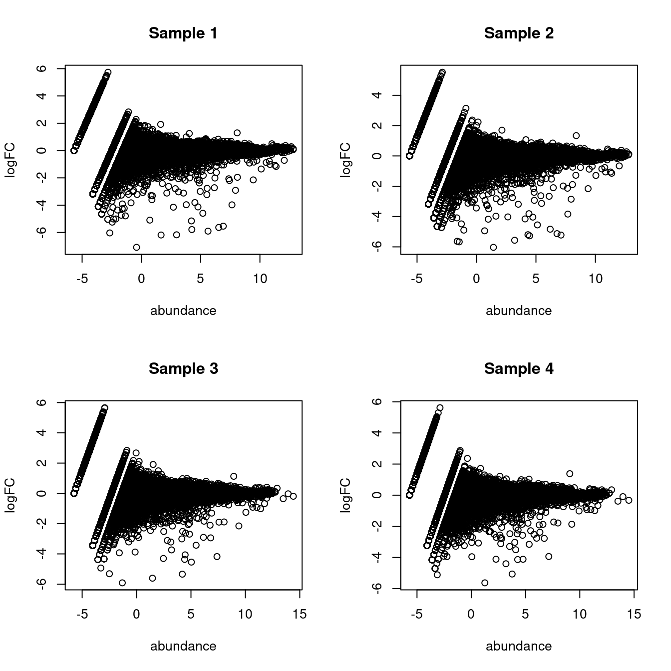
Figure 5.1: MA plots of the log-fold change of the proxy ambient profile over the real profile for each sample in the Tal1 chimera dataset.
Alternatively, we may choose to mitigate the effect of ambient contamination by focusing on label-specific DEGs. Contamination-driven DEGs should be systematically present in comparisons for all labels, and thus can be eliminated by simply ignoring all genes that are significant in a majority of these comparisons (Section 4.5.2). The obvious drawback of this approach is that it discounts genuine DEGs that have a consistent effect in most/all labels, though one could perhaps argue that such “global” DEGs are not particularly interesting anyway. It is also complicated by fluctuations in detection power across comparisons involving different numbers of cells - or replicates, after filtering pseudo-bulk profiles by the number of cells.
res.tal1 <- pseudoBulkSpecific(summed.tal1,
    label=summed.tal1$label,
    design=~factor(block) + tomato,
    coef="tomatoTRUE",
    condition=summed.tal1$tomato)

# Inspecting our neural crest results again.
tab.neural.again <- res.tal1[["Neural crest"]]
head(tab.neural.again[order(tab.neural.again$PValue),], 10)
## DataFrame with 10 rows and 6 columns
## logFC logCPM F PValue FDR
## <numeric> <numeric> <numeric> <numeric> <numeric>
## Fdps 0.981388 7.21805 337.1586 3.67655e-74 3.91553e-70
## Msmo1 1.493771 5.43923 301.0658 3.12891e-64 1.66614e-60
## Hmgcs1 1.250024 5.70837 252.1105 3.95670e-56 1.40463e-52
## Idi1 1.173709 5.37688 180.8890 6.68049e-41 1.77868e-37
## Gt(ROSA)26Sor 1.481294 5.71617 351.9402 2.50809e-32 5.34222e-29
## Sox9 0.537460 7.17373 99.3336 2.69822e-23 4.78934e-20
## Nkd1 0.719043 5.92690 93.9636 2.74595e-20 4.17777e-17
## Fdft1 0.841061 5.32293 89.8826 1.03053e-19 1.37189e-16
## Insig1 1.257339 4.06887 82.2931 1.37966e-19 1.63260e-16
## Acat2 0.508862 6.80012 73.8163 9.77138e-18 1.00391e-14
## OtherAverage
## <numeric>
## Fdps -0.0913554
## Msmo1 0.0269652
## Hmgcs1 -0.0628281
## Idi1 -0.0820383
## Gt(ROSA)26Sor 0.5412288
## Sox9 -0.0419813
## Nkd1 0.0332706
## Fdft1 0.0336446
## Insig1 -0.2899829
## Acat2 -0.0522834## DataFrame with 8 rows and 6 columns
## logFC logCPM F PValue FDR OtherAverage
## <numeric> <numeric> <numeric> <numeric> <numeric> <numeric>
## Hbb-bt -7.76718 1.33059 58.7089 1.000000 1.000000 -7.86812
## Hbb-bs -5.84817 3.42835 238.2627 1.000000 1.000000 -8.15469
## Hbb-bh2 NA NA NA NA NA -8.98446
## Hbb-bh1 -8.09104 9.15972 10758.2563 0.937101 1.000000 -8.08037
## Hbb-y -8.41562 8.35705 7364.2897 0.502375 1.000000 -8.21261
## Hba-x -7.72480 8.53284 7896.4567 0.138483 0.940591 -7.38504
## Hba-a1 -8.59671 6.74429 2756.5730 0.326266 1.000000 -8.05722
## Hba-a2 -8.86623 5.81300 1517.7259 0.254178 1.000000 -7.96508The common theme here is that, in the absence of an ambient profile, we are using all labels as a proxy for the ambient effect.
This can have unpredictable consequences as the results for each label are now dependent on the behavior of the entire dataset.
For example, the metrics are susceptible to the idiosyncrasies of clustering where one cell type may be represented in multple related clusters that distort the percentages in up.de and down.de or the average log-fold change.
The metrics may also be invalidated in analyses of a subset of the data - for example, a subclustering analysis focusing on a particular cell type may mark all relevant DEGs as problematic because they are consistently DE in all subtypes.
5.3 Subtracting ambient counts
It is worth commenting on the seductive idea of subtracting the ambient counts from the pseudo-bulk samples. This may seem like the most obvious approach for removing ambient contamination, but unfortunately, subtracted counts have unpredictable statistical properties due the distortion of the mean-variance relationship. Minor relative fluctuations at very large counts become large fold-changes after subtraction, manifesting as spurious DE in genes where a substantial proportion of counts is derived from the ambient solution. For example, several hemoglobin genes retain strong DE even after subtraction of the scaled ambient profile.
scaled.ambient <- controlAmbience(counts(summed.neural), ambient,
    features=is.hbb,  mode="profile")
subtracted <- counts(summed.neural) - scaled.ambient
subtracted <- round(subtracted)
subtracted[subtracted < 0] <- 0
subtracted[is.hbb,]
## [,1] [,2] [,3] [,4]
## Hbb-bt 0 0 7 18
## Hbb-bs 1 2 31 42
## Hbb-bh2 0 0 0 0
## Hbb-bh1 2 0 0 0
## Hbb-y 0 0 39 107
## Hba-x 1 1 0 0
## Hba-a1 0 0 365 452
## Hba-a2 0 0 314 329Another tempting approach is to use interaction models to implicitly subtract the ambient effect during GLM fitting. The assumption is that, for a genuine DEG, the log-fold change within cells is larger in magnitude than that in the ambient solution. This is based on the expectation that any DE in the latter is “diluted” by contributions from cell types where that gene is not DE. Unfortunately, this is not always the case; a DE analysis of the ambient counts indicates that the hemoglobin log-fold change is actually stronger in the neural crest cells compared to the ambient solution, which leads to the rather awkward conclusion that the WT neural crest cells are expressing hemoglobin beyond that explained by ambient contamination. (This is probably an artifact of how cell calling is performed.)
library(edgeR)
y.ambient <- DGEList(ambient, samples=colData(summed.neural))
y.ambient <- y.ambient[filterByExpr(y.ambient, group=y.ambient$samples$tomato),]
y.ambient <- calcNormFactors(y.ambient)

design <- model.matrix(~factor(block) + tomato, y.ambient$samples)
y.ambient <- estimateDisp(y.ambient, design)
fit.ambient <- glmQLFit(y.ambient, design, robust=TRUE)
res.ambient <- glmQLFTest(fit.ambient, coef=ncol(design))

summary(decideTests(res.ambient))
## tomatoTRUE
## Down 1910
## NotSig 7683
## Up 1645## Coefficient: tomatoTRUE
## logFC logCPM F PValue FDR
## Hbb-y -5.267 12.803 15115 3.523e-81 3.959e-77
## Hbb-bh1 -5.075 13.725 14002 8.892e-80 4.996e-76
## Hba-x -4.827 13.122 13317 3.135e-79 1.175e-75
## Hba-a1 -4.662 10.734 11095 1.146e-76 3.220e-73
## Hba-a2 -4.521 9.480 8411 1.246e-72 2.800e-69
## Blvrb -4.319 7.649 4129 3.066e-62 5.742e-59
## Xist -4.376 7.484 3891 1.864e-61 2.993e-58
## Gypa -5.138 7.213 3808 3.833e-61 5.384e-58
## Hbb-bs -4.941 7.209 3604 3.728e-60 4.655e-57
## Car2 -3.499 8.534 4448 5.589e-60 6.281e-57In addition, there are other issues with implicit subtraction in the fitted GLM that warrant caution with its use. This strategy precludes detection of DEGs that are common to all cell types as there is no longer a dilution effect being applied to the log-fold change in the ambient solution. It requires inclusion of the ambient profiles in the model, which is cause for at least some concern as they are unlikely to have the same degree of variability as the cell-derived pseudo-bulk profiles. Interpretation is also complicated by the fact that we are only interested in log-fold changes that are more extreme in the cells compared to the ambient solution; a non-zero interaction term is not sufficient for removing spurious DE.
See also comments in Advanced Section 7.3 for more comments on the removal of ambient contamination, mostly for visualization purposes.
Session Info
R version 4.1.0 beta (2021-05-03 r80259)
Platform: x86_64-pc-linux-gnu (64-bit)
Running under: Ubuntu 20.04.2 LTS

Matrix products: default
BLAS:   /home/biocbuild/bbs-3.14-bioc/R/lib/libRblas.so
LAPACK: /home/biocbuild/bbs-3.14-bioc/R/lib/libRlapack.so

locale:
 [1] LC_CTYPE=en_US.UTF-8       LC_NUMERIC=C
 [3] LC_TIME=en_GB              LC_COLLATE=C
 [5] LC_MONETARY=en_US.UTF-8    LC_MESSAGES=en_US.UTF-8
 [7] LC_PAPER=en_US.UTF-8       LC_NAME=C
 [9] LC_ADDRESS=C               LC_TELEPHONE=C
[11] LC_MEASUREMENT=en_US.UTF-8 LC_IDENTIFICATION=C

attached base packages:
[1] parallel  stats4    stats     graphics  grDevices utils     datasets
[8] methods   base

other attached packages:
 [1] edgeR_3.35.0                limma_3.49.0
 [3] DropletUtils_1.13.0         scran_1.21.1
 [5] scuttle_1.3.0               MouseGastrulationData_1.7.0
 [7] SpatialExperiment_1.3.0     SingleCellExperiment_1.15.1
 [9] SummarizedExperiment_1.23.0 Biobase_2.53.0
[11] GenomicRanges_1.45.0        GenomeInfoDb_1.29.0
[13] IRanges_2.27.0              S4Vectors_0.31.0
[15] BiocGenerics_0.39.0         MatrixGenerics_1.5.0
[17] matrixStats_0.58.0          BiocStyle_2.21.0
[19] rebook_1.3.0

loaded via a namespace (and not attached):
  [1] rjson_0.2.20                  ellipsis_0.3.2
  [3] bluster_1.3.0                 XVector_0.33.0
  [5] BiocNeighbors_1.11.0          bit64_4.0.5
  [7] interactiveDisplayBase_1.31.0 AnnotationDbi_1.55.0
  [9] fansi_0.4.2                   splines_4.1.0
 [11] codetools_0.2-18              R.methodsS3_1.8.1
 [13] sparseMatrixStats_1.5.0       cachem_1.0.5
 [15] knitr_1.33                    jsonlite_1.7.2
 [17] cluster_2.1.2                 dbplyr_2.1.1
 [19] png_0.1-7                     R.oo_1.24.0
 [21] graph_1.71.0                  shiny_1.6.0
 [23] HDF5Array_1.21.0              BiocManager_1.30.15
 [25] compiler_4.1.0                httr_1.4.2
 [27] dqrng_0.3.0                   assertthat_0.2.1
 [29] Matrix_1.3-3                  fastmap_1.1.0
 [31] later_1.2.0                   BiocSingular_1.9.0
 [33] htmltools_0.5.1.1             tools_4.1.0
 [35] igraph_1.2.6                  rsvd_1.0.5
 [37] glue_1.4.2                    GenomeInfoDbData_1.2.6
 [39] dplyr_1.0.6                   rappdirs_0.3.3
 [41] Rcpp_1.0.6                    jquerylib_0.1.4
 [43] vctrs_0.3.8                   Biostrings_2.61.0
 [45] rhdf5filters_1.5.0            ExperimentHub_2.1.0
 [47] DelayedMatrixStats_1.15.0     BumpyMatrix_1.1.0
 [49] xfun_0.23                     stringr_1.4.0
 [51] beachmat_2.9.0                irlba_2.3.3
 [53] mime_0.10                     lifecycle_1.0.0
 [55] statmod_1.4.36                XML_3.99-0.6
 [57] AnnotationHub_3.1.0           zlibbioc_1.39.0
 [59] promises_1.2.0.1              rhdf5_2.37.0
 [61] yaml_2.2.1                    curl_4.3.1
 [63] memoise_2.0.0                 sass_0.4.0
 [65] stringi_1.6.2                 RSQLite_2.2.7
 [67] highr_0.9                     BiocVersion_3.14.0
 [69] ScaledMatrix_1.1.0            filelock_1.0.2
 [71] BiocParallel_1.27.0           rlang_0.4.11
 [73] pkgconfig_2.0.3               bitops_1.0-7
 [75] evaluate_0.14                 lattice_0.20-44
 [77] purrr_0.3.4                   Rhdf5lib_1.15.0
 [79] CodeDepends_0.6.5             bit_4.0.4
 [81] tidyselect_1.1.1              magrittr_2.0.1
 [83] bookdown_0.22                 R6_2.5.0
 [85] magick_2.7.2                  generics_0.1.0
 [87] metapod_1.1.0                 DelayedArray_0.19.0
 [89] DBI_1.1.1                     pillar_1.6.1
 [91] withr_2.4.2                   KEGGREST_1.33.0
 [93] RCurl_1.98-1.3                tibble_3.1.2
 [95] dir.expiry_1.1.0              crayon_1.4.1
 [97] utf8_1.2.1                    BiocFileCache_2.1.0
 [99] rmarkdown_2.8                 locfit_1.5-9.4
[101] grid_4.1.0                    blob_1.2.1
[103] digest_0.6.27                 xtable_1.8-4
[105] httpuv_1.6.1                  R.utils_2.10.1
[107] bslib_0.2.5.1
References
Lun, A., S. Riesenfeld, T. Andrews, T. P. Dao, T. Gomes, participants in the 1st Human Cell Atlas Jamboree, and J. Marioni. 2019. “EmptyDrops: distinguishing cells from empty droplets in droplet-based single-cell RNA sequencing data.” Genome Biol. 20 (1): 63.
Pijuan-Sala, B., J. A. Griffiths, C. Guibentif, T. W. Hiscock, W. Jawaid, F. J. Calero-Nieto, C. Mulas, et al. 2019. “A Single-Cell Molecular Map of Mouse Gastrulation and Early Organogenesis.” Nature 566 (7745): 490–95.
Young, M. D., and S. Behjati. 2018. “SoupX Removes Ambient RNA Contamination from Droplet Based Single Cell RNA Sequencing Data.” bioRxiv.