Chapter 1 Quality control, redux
1.1 Overview
Basic Chapter 1 introduced the concept of per-cell quality control, focusing on outlier detection to provide an adaptive threshold on our chosen QC metrics. This chapter elaborates on the technical details of outlier-based quality control, including some of the underlying assumptions, how to handle multi-batch experiments and diagnosing loss of cell types. We will again demonstrate using the 416B dataset from A. T. L. Lun et al. (2017).
1.2 The isOutlier() function
The isOutlier() function from the scuttle package is the workhorse function for outlier detection.
As previously mentioned, it will define an observation as an outlier if it is more than a specified number of MADs (default 3) from the median in the specified direction.
library(AnnotationHub)
ens.mm.v97 <- AnnotationHub()[["AH73905"]]
chr.loc <- mapIds(ens.mm.v97, keys=rownames(sce.416b),
    keytype="GENEID", column="SEQNAME")
is.mito <- which(chr.loc=="MT")

library(scuttle)
df <- perCellQCMetrics(sce.416b, subsets=list(Mito=is.mito))
low.lib <- isOutlier(df$sum, type="lower", log=TRUE)
summary(low.lib)
## Mode FALSE TRUE
## logical 188 4## Mode FALSE TRUE
## logical 185 7The perCellQCFilters() function mentioned in Basic Chapter 1 is just a convenience wrapper around isOutlier().
Advanced users may prefer to use isOutlier() directly to achieve more control over the fields of df that are used for filtering.
reasons <- perCellQCFilters(df,
    sub.fields=c("subsets_Mito_percent", "altexps_ERCC_percent"))
stopifnot(identical(low.lib, reasons$low_lib_size))
We can also alter the directionality of the outlier detection, number of MADs used, as well as more advanced parameters related to batch processing (see Section 1.4). For example, we can remove both high and low outliers that are more than 5 MADs from the median. The output also contains the thresholds in the attributes for further perusal.
##  lower higher
## 434083    Inf
Incidentally, the is.mito code provides a demonstration of how to obtain the identity of the mitochondrial genes from the gene identifiers.
The same approach can be used for gene symbols by simply setting keytype="SYMBOL".
1.3 Assumptions of outlier detection
Outlier detection assumes that most cells are of acceptable quality. This is usually reasonable and can be experimentally supported in some situations by visually checking that the cells are intact, e.g., on the microwell plate. If most cells are of (unacceptably) low quality, the adaptive thresholds will fail as they cannot remove the majority of cells by definition - see Figure 1.1 below for a demonstrative example. Of course, what is acceptable or not is in the eye of the beholder - neurons, for example, are notoriously difficult to dissociate, and we would often retain cells in a neuronal scRNA-seq dataset with QC metrics that would be unacceptable in a more amenable system like embryonic stem cells.
Another assumption mentioned in Basic Chapter 1 is that the QC metrics are independent of the biological state of each cell. This is most likely to be violated in highly heterogeneous cell populations where some cell types naturally have, e.g., less total RNA (see Figure 3A of Germain, Sonrel, and Robinson (2020)) or more mitochondria. Such cells are more likely to be considered outliers and removed, even in the absence of any technical problems with their capture or sequencing. The use of the MAD mitigates this problem to some extent by accounting for biological variability in the QC metrics. A heterogeneous population should have higher variability in the metrics among high-quality cells, increasing the MAD and reducing the chance of incorrectly removing particular cell types (at the cost of reducing power to remove low-quality cells).
In general, these assumptions are either reasonable or their violations have little effect on downstream conclusions. Nonetheless, it is helpful to keep them in mind when interpreting the results.
1.4 Considering experimental factors
More complex studies may involve batches of cells generated with different experimental parameters (e.g., sequencing depth). In such cases, the adaptive strategy should be applied to each batch separately. It makes little sense to compute medians and MADs from a mixture distribution containing samples from multiple batches. For example, if the sequencing coverage is lower in one batch compared to the others, it will drag down the median and inflate the MAD. This will reduce the suitability of the adaptive threshold for the other batches.
If each batch is represented by its own SingleCellExperiment, the perCellQCFilters() function can be directly applied to each batch as previously described.
However, if cells from all batches have been merged into a single SingleCellExperiment, the batch= argument should be used to ensure that outliers are identified within each batch.
By doing so, the outlier detection algorithm has the opportunity to account for systematic differences in the QC metrics across batches.
Diagnostic plots are also helpful here: batches with systematically poor values for any metric can then be quickly identified for further troubleshooting or outright removal.
We will again illustrate using the 416B dataset, which contains two experimental factors - plate of origin and oncogene induction status.
We combine these factors together and use this in the batch= argument to isOutlier() via quickPerCellQC().
This results in the removal of slightly more cells as the MAD is no longer inflated by (i) systematic differences in sequencing depth between batches and (ii) differences in number of genes expressed upon oncogene induction.
batch <- paste0(sce.416b$phenotype, "-", sce.416b$block)
batch.reasons <- perCellQCFilters(df, batch=batch,
    sub.fields=c("subsets_Mito_percent", "altexps_ERCC_percent"))
colSums(as.matrix(batch.reasons))
## low_lib_size low_n_features high_subsets_Mito_percent
## 5 4 2
## high_altexps_ERCC_percent discard
## 6 9That said, the use of batch= involves the stronger assumption that most cells in each batch are of high quality.
If an entire batch failed, outlier detection will not be able to act as an appropriate QC filter for that batch.
For example, two batches in the Grun et al. (2016) human pancreas dataset contain a substantial proportion of putative damaged cells with higher ERCC content than the other batches (Figure 1.1).
This inflates the median and MAD within those batches, resulting in a failure to remove the assumed low-quality cells.
library(scRNAseq)
sce.grun <- GrunPancreasData()
sce.grun <- addPerCellQC(sce.grun)

# First attempt with batch-specific thresholds.
library(scater)
discard.ercc <- isOutlier(sce.grun$altexps_ERCC_percent,
    type="higher", batch=sce.grun$donor)
plotColData(sce.grun, x="donor", y="altexps_ERCC_percent",
    colour_by=I(discard.ercc))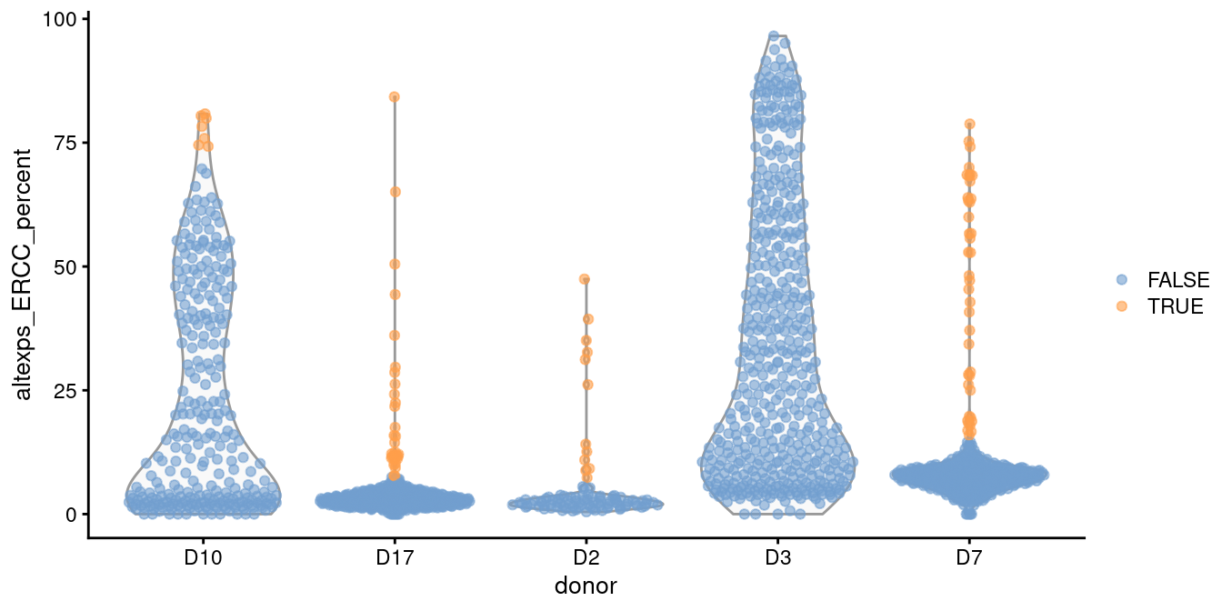
Figure 1.1: Distribution of the proportion of ERCC transcripts in each donor of the Grun pancreas dataset. Each point represents a cell and is coloured according to whether it was identified as an outlier within each batch.
In such cases, it is better to compute a shared median and MAD from the other batches and use those estimates to obtain an appropriate filter threshold for cells in the problematic batches.
This is automatically done by isOutlier() when we susbet to cells from those other batches, as shown in Figure 1.2.
# Second attempt, sharing information across batches
# to avoid dramatically different thresholds for unusual batches.
discard.ercc2 <- isOutlier(sce.grun$altexps_ERCC_percent,
    type="higher", batch=sce.grun$donor,
    subset=sce.grun$donor %in% c("D17", "D2", "D7"))

plotColData(sce.grun, x="donor", y="altexps_ERCC_percent",
    colour_by=I(discard.ercc2))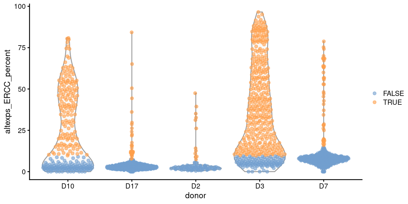
Figure 1.2: Distribution of the proportion of ERCC transcripts in each donor of the Grun pancreas dataset. Each point represents a cell and is coloured according to whether it was identified as an outlier, using a common threshold for the problematic batches.
To identify problematic batches, one useful rule of thumb is to find batches with QC thresholds that are themselves outliers compared to the thresholds of other batches. The assumption here is that most batches consist of a majority of high quality cells such that the threshold value should follow some unimodal distribution across “typical” batches. If we observe a batch with an extreme threshold value, we may suspect that it contains a large number of low-quality cells that inflate the per-batch MAD. We demonstrate this process below for the Grun et al. (2016) data.
##     D10     D17      D2      D3      D7
## 73.611 7.600 6.011 113.106 15.217## [1] "D10" "D3"If we cannot assume that most batches contain a majority of high-quality cells, then all bets are off; we must revert to the approach of picking an arbitrary threshold value (Basic Section 1.3.1) based on some “sensible” prior expectations and hoping for the best.
1.5 Diagnosing cell type loss
The biggest practical concern during QC is whether an entire cell type is inadvertently discarded. There is always some risk of this occurring as the QC metrics are never fully independent of biological state. We can diagnose cell type loss by looking for systematic differences in gene expression between the discarded and retained cells. To demonstrate, we compute the average count across the discarded and retained pools in the 416B data set, and we compute the log-fold change between the pool averages.
# Using the non-batched 'discard' vector for demonstration purposes,
# as it has more cells for stable calculation of 'lost'.
discard <- reasons$discard
lost <- calculateAverage(counts(sce.416b)[,!discard])
kept <- calculateAverage(counts(sce.416b)[,discard])

library(edgeR)
logged <- cpm(cbind(lost, kept), log=TRUE, prior.count=2)
logFC <- logged[,1] - logged[,2]
abundance <- rowMeans(logged)
If the discarded pool is enriched for a certain cell type, we should observe increased expression of the corresponding marker genes. No systematic upregulation of genes is apparent in the discarded pool in Figure 1.3, suggesting that the QC step did not inadvertently filter out a cell type in the 416B dataset.
plot(abundance, logFC, xlab="Average count", ylab="Log-FC (lost/kept)", pch=16)
points(abundance[is.mito], logFC[is.mito], col="dodgerblue", pch=16)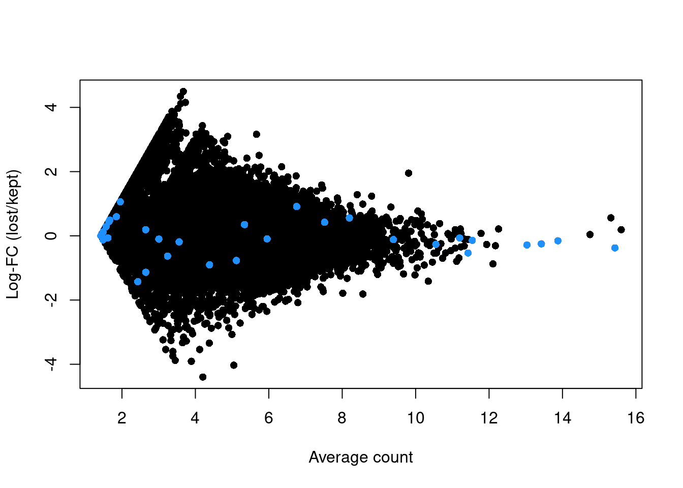
Figure 1.3: Log-fold change in expression in the discarded cells compared to the retained cells in the 416B dataset. Each point represents a gene with mitochondrial transcripts in blue.
For comparison, let us consider the QC step for the PBMC dataset from 10X Genomics (Zheng et al. 2017). We’ll apply an arbitrary fixed threshold on the library size to filter cells rather than using any outlier-based method. Specifically, we remove all libraries with a library size below 500.
#--- loading ---#
library(DropletTestFiles)
raw.path <- getTestFile("tenx-2.1.0-pbmc4k/1.0.0/raw.tar.gz")
out.path <- file.path(tempdir(), "pbmc4k")
untar(raw.path, exdir=out.path)

library(DropletUtils)
fname <- file.path(out.path, "raw_gene_bc_matrices/GRCh38")
sce.pbmc <- read10xCounts(fname, col.names=TRUE)

#--- gene-annotation ---#
library(scater)
rownames(sce.pbmc) <- uniquifyFeatureNames(
    rowData(sce.pbmc)$ID, rowData(sce.pbmc)$Symbol)

library(EnsDb.Hsapiens.v86)
location <- mapIds(EnsDb.Hsapiens.v86, keys=rowData(sce.pbmc)$ID,
    column="SEQNAME", keytype="GENEID")

#--- cell-detection ---#
set.seed(100)
e.out <- emptyDrops(counts(sce.pbmc))
sce.pbmc <- sce.pbmc[,which(e.out$FDR <= 0.001)]
discard <- colSums(counts(sce.pbmc)) < 500
lost <- calculateAverage(counts(sce.pbmc)[,discard])
kept <- calculateAverage(counts(sce.pbmc)[,!discard])
logged <- edgeR::cpm(cbind(lost, kept), log=TRUE, prior.count=2)
logFC <- logged[,1] - logged[,2]
abundance <- rowMeans(logged)The presence of a distinct population in the discarded pool manifests in Figure 1.4 as a set of genes that are strongly upregulated in lost.
This includes PF4, PPBP and SDPR, which (spoiler alert!) indicates that there is a platelet population that has been discarded by alt.discard.
plot(abundance, logFC, xlab="Average count", ylab="Log-FC (lost/kept)", pch=16)
platelet <- c("PF4", "PPBP", "SDPR")
points(abundance[platelet], logFC[platelet], col="orange", pch=16)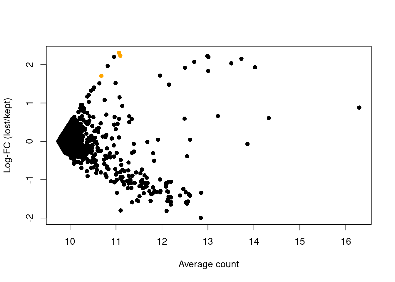
Figure 1.4: Average counts across all discarded and retained cells in the PBMC dataset, after using a more stringent filter on the total UMI count. Each point represents a gene, with platelet-related genes highlighted in orange.
If we suspect that cell types have been incorrectly discarded by our QC procedure, the most direct solution is to relax the QC filters for metrics that are associated with genuine biological differences.
For example, outlier detection can be relaxed by increasing nmads= in the isOutlier() calls.
Of course, this increases the risk of retaining more low-quality cells and encountering the problems discussed in Basic Section 1.1.
The logical endpoint of this line of reasoning is to avoid filtering altogether, as discussed in Basic Section 1.5.
As an aside, it is worth mentioning that the true technical quality of a cell may also be correlated with its type. (This differs from a correlation between the cell type and the QC metrics, as the latter are our imperfect proxies for quality.) This can arise if some cell types are not amenable to dissociation or microfluidics handling during the scRNA-seq protocol. In such cases, it is possible to “correctly” discard an entire cell type during QC if all of its cells are damaged. Indeed, concerns over the computational removal of cell types during QC are probably minor compared to losses in the experimental protocol.
Session Info
R version 4.1.2 (2021-11-01)
Platform: x86_64-pc-linux-gnu (64-bit)
Running under: Ubuntu 20.04.3 LTS

Matrix products: default
BLAS:   /home/biocbuild/bbs-3.14-bioc/R/lib/libRblas.so
LAPACK: /home/biocbuild/bbs-3.14-bioc/R/lib/libRlapack.so

locale:
 [1] LC_CTYPE=en_US.UTF-8       LC_NUMERIC=C
 [3] LC_TIME=en_GB              LC_COLLATE=C
 [5] LC_MONETARY=en_US.UTF-8    LC_MESSAGES=en_US.UTF-8
 [7] LC_PAPER=en_US.UTF-8       LC_NAME=C
 [9] LC_ADDRESS=C               LC_TELEPHONE=C
[11] LC_MEASUREMENT=en_US.UTF-8 LC_IDENTIFICATION=C

attached base packages:
[1] stats4    stats     graphics  grDevices utils     datasets  methods
[8] base

other attached packages:
 [1] edgeR_3.36.0                limma_3.50.0
 [3] scater_1.22.0               ggplot2_3.3.5
 [5] scRNAseq_2.8.0              scuttle_1.4.0
 [7] SingleCellExperiment_1.16.0 SummarizedExperiment_1.24.0
 [9] MatrixGenerics_1.6.0        matrixStats_0.61.0
[11] ensembldb_2.18.2            AnnotationFilter_1.18.0
[13] GenomicFeatures_1.46.1      AnnotationDbi_1.56.2
[15] Biobase_2.54.0              GenomicRanges_1.46.0
[17] GenomeInfoDb_1.30.0         IRanges_2.28.0
[19] S4Vectors_0.32.2            AnnotationHub_3.2.0
[21] BiocFileCache_2.2.0         dbplyr_2.1.1
[23] BiocGenerics_0.40.0         BiocStyle_2.22.0
[25] rebook_1.4.0

loaded via a namespace (and not attached):
  [1] lazyeval_0.2.2                BiocParallel_1.28.0
  [3] digest_0.6.28                 htmltools_0.5.2
  [5] viridis_0.6.2                 fansi_0.5.0
  [7] magrittr_2.0.1                memoise_2.0.0
  [9] ScaledMatrix_1.2.0            Biostrings_2.62.0
 [11] prettyunits_1.1.1             colorspace_2.0-2
 [13] blob_1.2.2                    rappdirs_0.3.3
 [15] ggrepel_0.9.1                 xfun_0.28
 [17] dplyr_1.0.7                   crayon_1.4.2
 [19] RCurl_1.98-1.5                jsonlite_1.7.2
 [21] graph_1.72.0                  glue_1.5.0
 [23] gtable_0.3.0                  zlibbioc_1.40.0
 [25] XVector_0.34.0                DelayedArray_0.20.0
 [27] BiocSingular_1.10.0           scales_1.1.1
 [29] DBI_1.1.1                     Rcpp_1.0.7
 [31] viridisLite_0.4.0             xtable_1.8-4
 [33] progress_1.2.2                bit_4.0.4
 [35] rsvd_1.0.5                    httr_1.4.2
 [37] dir.expiry_1.2.0              ellipsis_0.3.2
 [39] pkgconfig_2.0.3               XML_3.99-0.8
 [41] farver_2.1.0                  CodeDepends_0.6.5
 [43] sass_0.4.0                    locfit_1.5-9.4
 [45] utf8_1.2.2                    tidyselect_1.1.1
 [47] labeling_0.4.2                rlang_0.4.12
 [49] later_1.3.0                   munsell_0.5.0
 [51] BiocVersion_3.14.0            tools_4.1.2
 [53] cachem_1.0.6                  generics_0.1.1
 [55] RSQLite_2.2.8                 ExperimentHub_2.2.0
 [57] evaluate_0.14                 stringr_1.4.0
 [59] fastmap_1.1.0                 yaml_2.2.1
 [61] knitr_1.36                    bit64_4.0.5
 [63] purrr_0.3.4                   KEGGREST_1.34.0
 [65] sparseMatrixStats_1.6.0       mime_0.12
 [67] xml2_1.3.2                    biomaRt_2.50.0
 [69] compiler_4.1.2                beeswarm_0.4.0
 [71] filelock_1.0.2                curl_4.3.2
 [73] png_0.1-7                     interactiveDisplayBase_1.32.0
 [75] tibble_3.1.6                  bslib_0.3.1
 [77] stringi_1.7.5                 highr_0.9
 [79] lattice_0.20-45               ProtGenerics_1.26.0
 [81] Matrix_1.3-4                  vctrs_0.3.8
 [83] pillar_1.6.4                  lifecycle_1.0.1
 [85] BiocManager_1.30.16           jquerylib_0.1.4
 [87] BiocNeighbors_1.12.0          cowplot_1.1.1
 [89] bitops_1.0-7                  irlba_2.3.3
 [91] httpuv_1.6.3                  rtracklayer_1.54.0
 [93] R6_2.5.1                      BiocIO_1.4.0
 [95] bookdown_0.24                 promises_1.2.0.1
 [97] gridExtra_2.3                 vipor_0.4.5
 [99] codetools_0.2-18              assertthat_0.2.1
[101] rjson_0.2.20                  withr_2.4.2
[103] GenomicAlignments_1.30.0      Rsamtools_2.10.0
[105] GenomeInfoDbData_1.2.7        parallel_4.1.2
[107] hms_1.1.1                     grid_4.1.2
[109] beachmat_2.10.0               rmarkdown_2.11
[111] DelayedMatrixStats_1.16.0     shiny_1.7.1
[113] ggbeeswarm_0.6.0              restfulr_0.0.13
References
Germain, P. L., A. Sonrel, and M. D. Robinson. 2020. “pipeComp, a general framework for the evaluation of computational pipelines, reveals performant single cell RNA-seq preprocessing tools.” Genome Biol. 21 (1): 227.
Grun, D., M. J. Muraro, J. C. Boisset, K. Wiebrands, A. Lyubimova, G. Dharmadhikari, M. van den Born, et al. 2016. “De Novo Prediction of Stem Cell Identity using Single-Cell Transcriptome Data.” Cell Stem Cell 19 (2): 266–77.
Lun, A. T. L., F. J. Calero-Nieto, L. Haim-Vilmovsky, B. Gottgens, and J. C. Marioni. 2017. “Assessing the reliability of spike-in normalization for analyses of single-cell RNA sequencing data.” Genome Res. 27 (11): 1795–1806.
Zheng, G. X., J. M. Terry, P. Belgrader, P. Ryvkin, Z. W. Bent, R. Wilson, S. B. Ziraldo, et al. 2017. “Massively parallel digital transcriptional profiling of single cells.” Nat Commun 8 (January): 14049.