Chapter 20 Integrating with protein abundance
20.1 Motivation
Cellular indexing of transcriptomes and epitopes by sequencing (CITE-seq) is a technique that quantifies both gene expression and the abundance of selected surface proteins in each cell simultaneously (Stoeckius et al. 2017). In this approach, cells are first labelled with antibodies that have been conjugated to synthetic RNA tags. A cell with a higher abundance of a target protein will be bound by more antibodies, causing more molecules of the corresponding antibody-derived tag (ADT) to be attached to that cell. Cells are then separated into their own reaction chambers using droplet-based microfluidics (Zheng et al. 2017). Both the ADTs and endogenous transcripts are reverse-transcribed and captured into a cDNA library; the abundance of each protein or expression of each gene is subsequently quantified by sequencing of each set of features. This provides a powerful tool for interrogating aspects of the proteome (such as post-translational modifications) and other cellular features that would normally be invisible to transcriptomic studies.
How should the ADT data be incorporated into the analysis? While we have counts for both ADTs and transcripts, there are fundamental differences in nature of the data that make it difficult to treat the former as additional features in the latter. Most experiments involve only a small number of antibodies (<20) that are chosen by the researcher because they are of a priori interest, in contrast to gene expression data that captures the entire transcriptome regardless of the study. The coverage of the ADTs is also much deeper as they are sequenced separately from the transcripts, allowing the sequencing resources to be concentrated into a smaller number of features. And, of course, the use of antibodies against protein targets involves consideration of separate biases compared to those observed for transcripts.
In this chapter, we will describe some strategies for integrated analysis of ADT and transcript data in CITE-seq experiments.
We will demonstrate using a PBMC dataset from 10X Genomics that contains quantified abundances for a number of interesting surface proteins.
We conveniently obtain the dataset using the DropletTestFiles package, after which we can create a SingleCellExperiment as shown below.
library(DropletTestFiles)
path <- getTestFile("tenx-3.0.0-pbmc_10k_protein_v3/1.0.0/filtered.tar.gz")
dir <- tempfile()
untar(path, exdir=dir)

# Loading it in as a SingleCellExperiment object.
library(DropletUtils)
sce <- read10xCounts(file.path(dir, "filtered_feature_bc_matrix"))
sce
## class: SingleCellExperiment
## dim: 33555 7865
## metadata(1): Samples
## assays(1): counts
## rownames(33555): ENSG00000243485 ENSG00000237613 ... IgG1 IgG2b
## rowData names(3): ID Symbol Type
## colnames: NULL
## colData names(2): Sample Barcode
## reducedDimNames(0):
## altExpNames(0):20.2 Setting up the data
The SingleCellExperiment class provides the concept of an “alternative Experiment” to store data for different sets of features but the same cells.
This involves storing another SummarizedExperiment (or an instance of a subclass) inside our SingleCellExperiment where the rows (features) can differ but the columns (cells) are the same.
In previous chapters, we were using the alternative Experiments to store spike-in data, but here we will use the concept to split off the ADT data.
This isolates the two sets of features to ensure that analyses on one set do not inadvertently use data from the other set, and vice versa.
## [1] "Antibody Capture"## class: SingleCellExperiment
## dim: 17 7865
## metadata(1): Samples
## assays(1): counts
## rownames(17): CD3 CD4 ... IgG1 IgG2b
## rowData names(3): ID Symbol Type
## colnames: NULL
## colData names(0):
## reducedDimNames(0):
## altExpNames(0):At this point, it is also helpful to coerce the sparse matrix for ADTs into a dense matrix. The ADT counts are usually not sparse so storage as a sparse matrix provides no advantage; in fact, it actually increases memory usage and computational time as the indices of non-zero entries must be unnecessarily stored and processed. From a practical perspective, this avoids unnecessary incompatibilities with downstream applications that do not accept sparse inputs.
##        [,1] [,2] [,3] [,4] [,5] [,6] [,7] [,8] [,9] [,10]
## CD3      18   30   18   18    5   21   34   48 4522  2910
## CD4     138  119  207   11   14 1014  324 1127 3479  2900
## CD8a     13   19   10   17   14   29   27   43   38    28
## CD14    491  472 1289   20   19 2428 1958 2189   55    41
## CD15     61  102  128  124  156  204  607  128  111   130
## CD16     17  155   72 1227 1873  148  676   75   44    37
## CD56     17  248   26  491  458   29   29   29   30    15
## CD19      3    3    8    5    4    7   15    4    6     6
## CD25      9    5   15   15   16   52   85   17   13    18
## CD45RA  110  125 5268 4743 4108  227  175  523 4044  1081
## CD45RO   74  156   28   28   21  492  517  316   26    43
## PD-1      9    9   20   25   28   16   26   16   28    16
## TIGIT     4    9   11   59   76   11   12   12    9     8
## CD127     7    8   12   16   17   15   11   10  231   179
## IgG2a     5    4   12   12    7    9    6    3   19    14
## IgG1      2    8   19   16   14   10   12    7   16    10
## IgG2b     3    3    6    4    9    8   50    2    8     2
20.3 Quality control
As with the endogenous genes, we want to remove cells that have failed to capture/sequence the ADTs. Recall that droplet-based libraries will contain contamination from ambient solution (Section 15.2), in this case containing containing conjugated antibodies that are either free in solution or bound to cell fragments. As the ADTs are (relatively) deeply sequenced, we can expect non-zero counts for most ADTs in each cell due to contamination (Figure 20.1; if this is not the case, we might suspect some failure of ADT processing for that cell. We thus remove cells that have unusually low numbers of detected ADTs, defined here as less than or equal to half of the total number of tags.
# Applied on the alternative experiment containing the ADT counts:
library(scuttle)
df.ab <- perCellQCMetrics(altExp(sce))

n.nonzero <- sum(!rowAlls(counts(altExp(sce)), value=0L))
ab.discard <- df.ab$detected <= n.nonzero/2
summary(ab.discard)
## Mode FALSE TRUE
## logical 7864 1hist(df.ab$detected, col='grey', main="", xlab="Number of detected ADTs")
abline(v=n.nonzero/2, col="red", lty=2)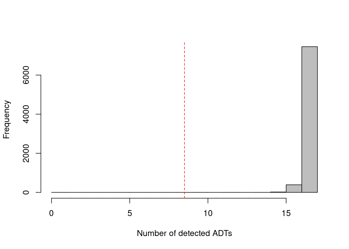
Figure 20.1: Distribution of the number of detected ADTs across all cells in the PBMC dataset. The red dotted line indicates the threshold below which cells were removed.
To elaborate on the filter above: we use n.nonzero to exclude ADTs with zero counts across all cells, which avoids inflation of the total number of ADTs due to barcodes that were erroniously included in the annotation.
The use of the specific threshold of 50% aims to avoid zero size factors during median-based normalization (Section 20.4.3), though it is straightforward to use more stringent thresholds if so desired.
We do not rely only on isOutlier() as the MAD is often zero in deeply sequenced datasets - where most cells contain non-zero counts for all ADTs - such that filtering would discard useful cells that only detect almost all of the ADTs.
Some experiments include isotype control (IgG) antibodies that have similar properties to a primary antibody but lack a specific target in the cell, thus providing a measure of non-specific binding. If we assume that the magnitude of non-specific binding is constant across cells, we could define low-quality cells as those with unusually low coverage of the control ADTs, presumably due to failed capture or sequencing. We use the outlier-based approach described in Chapter 6 to choose an appropriate filter threshold (Figure 20.2); hard thresholds are more difficult to specify due to experiment-by-experiment variation in the expected coverage of ADTs. Paradoxically, though, this QC metric becomes less useful in well-executed experiments where there is not enough non-specific binding to obtain meaningful coverage of the control ADTs.
# We could have specified subsets= in the above perCellQCMetrics call, but it's
# easier to explain one concept at a time, so we'll just repeat it here:
controls <- grep("^Ig", rownames(altExp(sce)))
df.ab2 <- perCellQCMetrics(altExp(sce), subsets=list(controls=controls))

con.discard <- isOutlier(df.ab2$subsets_controls_sum, log=TRUE, type="lower")
summary(con.discard)
## Mode FALSE TRUE
## logical 7785 80hist(log1p(df.ab2$subsets_controls_sum), col='grey', breaks=50,
main="", xlab="Log-total count for controls per cell")
abline(v=log1p(attr(con.discard, "thresholds")["lower"]), col="red", lty=2)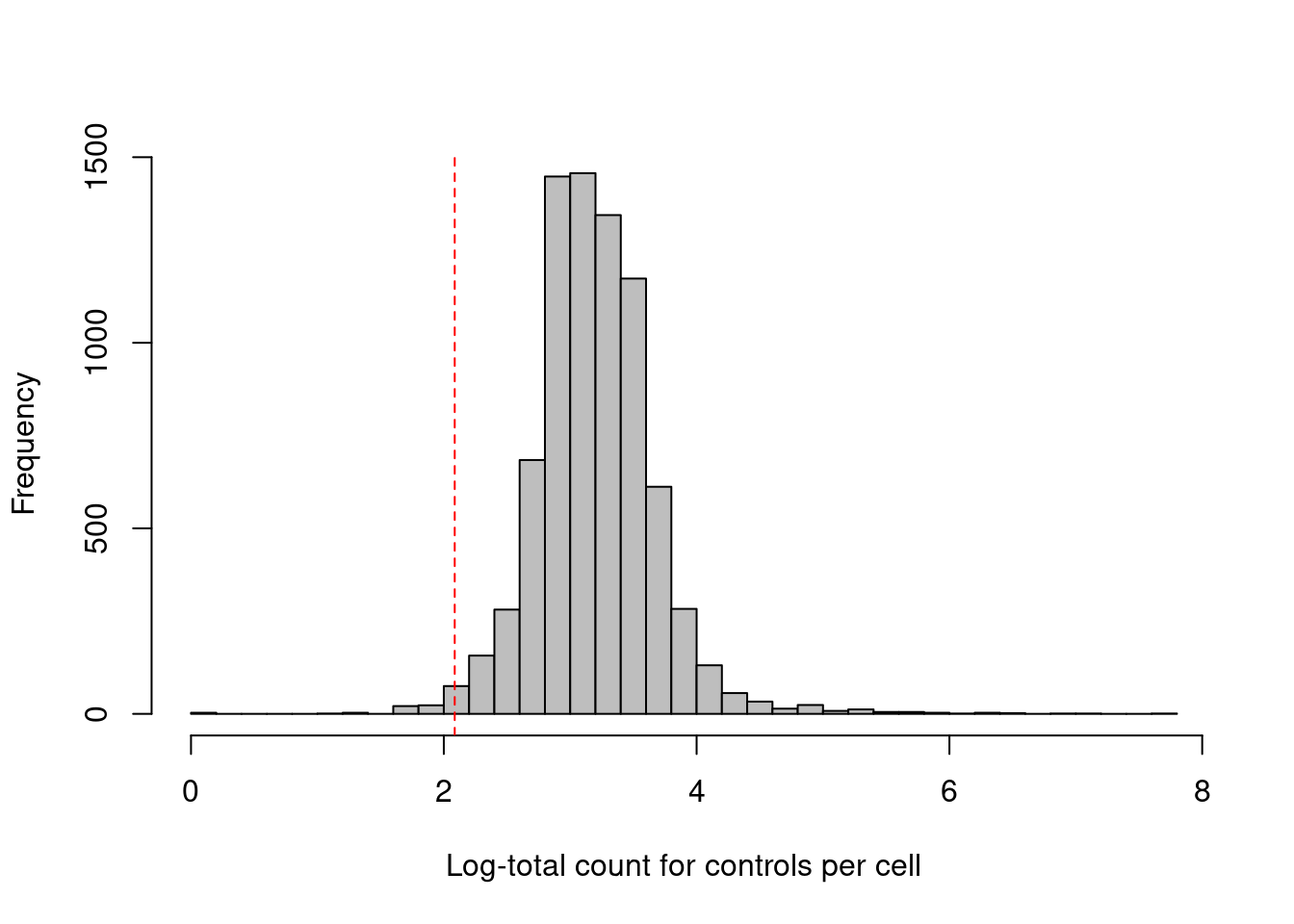
Figure 20.2: Distribution of the log-coverage of IgG control ADTs across all cells in the PBMC dataset. The red dotted line indicates the threshold below which cells were removed.
As with scRNA-seq, the total count across all ADTs can also be used as a QC metric (Figure 20.3). However, it is a riskier proportion for CITE-seq as there is a greater risk that the total count will be strongly correlated with the biological state of the cell. The presence of a targeted protein can lead to a several-fold increase in the total ADT count given the binary nature of most surface protein markers. Removing cells with low totals could inadvertently eliminate cell types that do not express many - or indeed, any - of the selected protein targets. Admittedly, this problem is the same as that discussed previously for the library size in scRNA-seq data (Section 6.3.2.2) but can be more pronounced in CITE-seq where there is no guaranteed set of constitutively expressed features to “buffer” cell-type-specific variation in the total count.
##    Mode   FALSE    TRUE
## logical 7820 45hist(log1p(df.ab2$sum), col='grey', breaks=50, main="", xlab="Log-total count per cell")
abline(v=log1p(attr(sum.discard, "thresholds")["lower"]), col="red", lty=2)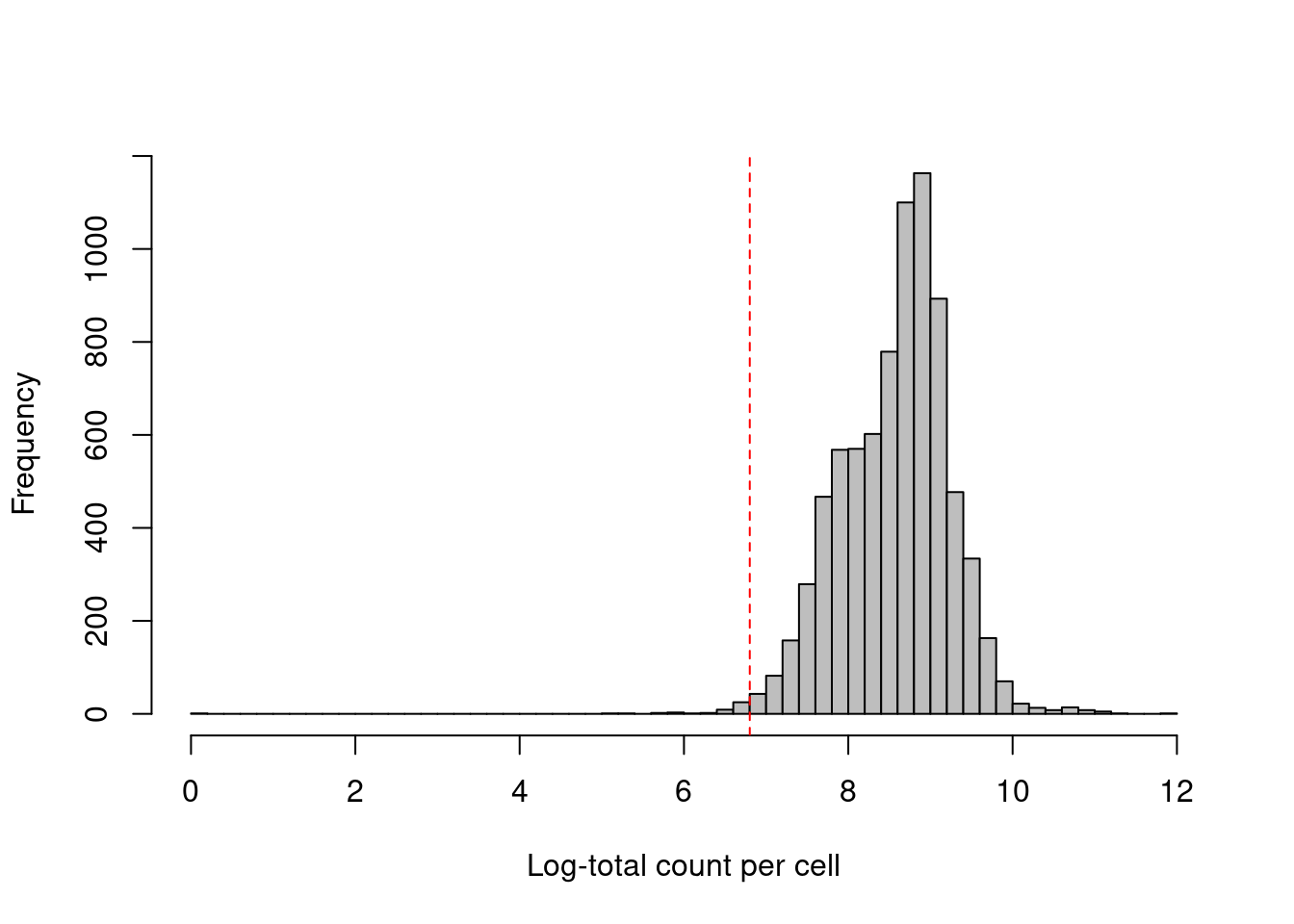
Figure 20.3: Distribution of the log-total count of all ADTs across all cells in the PBMC dataset. The red dotted line indicates the threshold below which cells are considered to be low outliers.
Of course, if we want to analyze gene expression and ADT data together, we still need to apply quality control on the gene counts. It is possible for a cell to have satisfactory ADT counts but poor QC metrics from the endogenous genes - for example, cell damage manifesting as high mitochondrial proportions would not be captured in the ADT data. More generally, the ADTs are synthetic, external to the cell and conjugated to antibodies, so it is not surprising that they would experience different cell-specific technical effects than the endogenous transcripts. This motivates a distinct QC step on the genes to ensure that we only retain high-quality cells in both feature spaces. Here, the count matrix has already been filtered by Cellranger to remove empty droplets so we only filter on the mitochondrial proportions to remove putative low-quality cells.
mito <- grep("^MT-", rowData(sce)$Symbol)
df <- perCellQCMetrics(sce, subsets=list(Mito=mito))
mito.discard <- isOutlier(df$subsets_Mito_percent, type="higher")
summary(mito.discard)
## Mode FALSE TRUE
## logical 7569 296Finally, to remove the low-quality cells, we subset the SingleCellExperiment as previously described.
This automatically applies the filtering to both the transcript and ADT data; such coordination is one of the advantages of storing both datasets in a single object.
We omit the total count filter to reduce the risk of discarding an all-negative cell type, at least for the first round of analysis.
20.4 Normalization
20.4.1 Overview
Counts for the ADTs are subject to several biases that must be normalized prior to further analysis. Capture efficiency varies from cell to cell though the differences in biophysical properties between endogenous transcripts and the (much shorter) ADTs means that the capture-related biases for the two sets of features are unlikely to be identical. Composition biases are also much more pronounced in ADT data due to (i) the binary nature of target protein abundances, where any increase in protein abundance manifests as a large increase to the total tag count; and (ii) the a priori selection of interesting protein targets, which enriches for features that are more likely to be differentially abundant across the population. As in Chapter 7, we assume that these are scaling biases and compute ADT-specific size factors to remove them. To this end, several strategies are again available to calculate a size factor for each cell.
20.4.2 Library size normalization
The simplest approach is to normalize on the total ADT counts, effectively the library size for the ADTs. Like in Section 7.2, these “ADT library size factors” are adequate for clustering but will introduce composition biases that interfere with interpretation of the fold-changes between clusters. This is especially tue for relatively subtle (e.g., ~2-fold) changes in the abundances of markers associated with functional activity rather than cell type.
##    Min. 1st Qu.  Median    Mean 3rd Qu.    Max.
##   0.031   0.528   0.906   1.000   1.266  22.672
We might instead consider the related approach of taking the geometric mean of all counts as the size factor for each cell (Stoeckius et al. 2017). The geometric mean is a reasonable estimator of the scaling biases for large counts with the added benefit that it mitigates the effects of composition biases by dampening the impact of one or two highly abundant ADTs. While more robust than the ADT library size factors, these geometric mean-based factors are still not entirely correct and will progressively become less accurate as upregulation increases in strength.
##    Min. 1st Qu.  Median    Mean 3rd Qu.    Max.
##    0.16    0.66    0.85    1.00    1.07   45.22
20.4.3 Median-based normalization
Ideally, we would like to compute size factors that adjust for the composition biases. This usually requires an assumption that most ADTs are not differentially expressed between cell types/states. At first glance, this appears to be a strong assumption - the target proteins were specifically chosen as they exhibit interesting heterogeneity across the population, meaning that a non-differential majority across ADTs would be unlikely. However, we can make it work by assuming that each cell only upregulates a minority of the targeted proteins, with the remaining ADTs exhibiting some low baseline abundance that is constant across all cells. (Of course, the identity of the upregulated subset can differ across cells, otherwise the dataset would not be very interesting.) We then compute size factors to equalize the coverage of the non-upregulated majority, thus eliminating cell-to-cell differences in capture efficiency.
We consider the baseline ADT profile to be a combination of weak constitutive expression and ambient contamination, both of which should be constant across the population.
We estimate this profile by assuming that the distribution of abundances for each ADT should be bimodal, where one population of cells exhibits low baseline expression and another population upregulates the corresponding protein target.
We then use all cells in the lower mode to compute the baseline abundance for that ADT.
This entire calculation is performed by the inferAmbience() function, which was originally designed to estimate HTO ambient concentrations but can be repurposed for more general use (Figure 20.4).
##    CD3    CD4   CD8a   CD14   CD15   CD16
## 30.99 29.97 30.09 32.61 108.65 45.25library(scater)
plotExpression(altExp(sce), features=rownames(altExp(sce)), exprs_values="counts") +
scale_y_log10() +
geom_point(data=data.frame(x=names(baseline), y=baseline), mapping=aes(x=x, y=y), cex=3)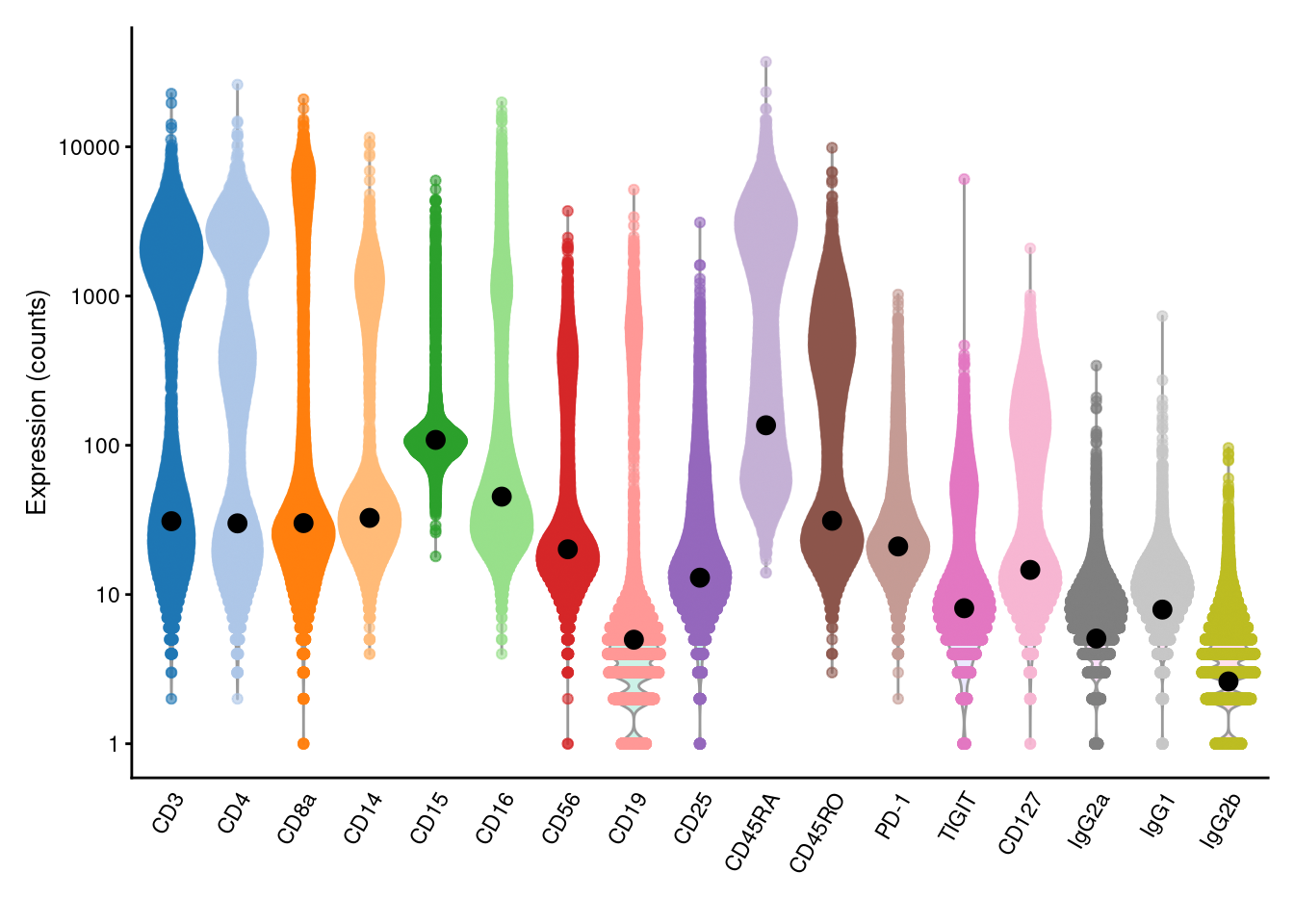
Figure 20.4: Distribution of (log-)counts for each ADT in the PBMC dataset, with the inferred ambient abundance marked by the black dot.
We use a DESeq2-like approach to compute size factors against the baseline profile. Specifically, the size factor for each cell is defined as the median of the ratios of that cell’s counts to the baseline profile. If the abundances for most ADTs in each cell are baseline-derived, they should be roughly constant across cells; any systematic differences in the ratios correspond to cell-specific biases in sequencing coverage and are captured by the size factor. The use of the median protects against the minority of ADTs corresponding to genuinely expressed targets.
##    Min. 1st Qu.  Median    Mean 3rd Qu.    Max.
##    0.20    0.66    0.78    1.00    1.00   71.00
In one subpopulation, the size factors are consistently larger than the ADT library size factors, whereas the opposite is true for most of the other subpopulations (Figure 20.5). This is consistent with the presence of composition biases due to differential abundance of the targeted proteins between subpopulations. Here, composition biases would introduce a spurious 2-fold change in normalized ADT abundance if the library size factors were used.
# Coloring by cluster to highlight the composition biases.
# We set k=20 to get fewer, broader clusters for a clearer picture.
library(scran)
tagdata <- logNormCounts(altExp(sce)) # library size factors by default.
g <- buildSNNGraph(tagdata, k=20, d=NA) # no need for PCA, see below.
clusters <- igraph::cluster_walktrap(g)$membership

plot(sf.lib, sf.amb, log="xy", col=clusters,
    xlab="Library size factors (tag)",
    ylab="DESeq-like size factors (tag)")
abline(0, 1, col="grey", lty=2)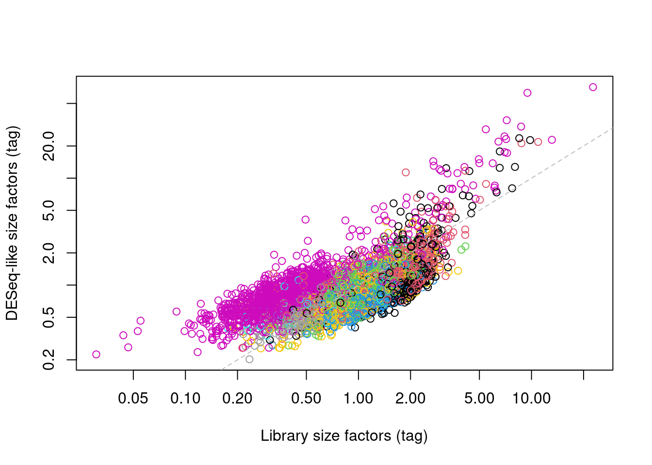
Figure 20.5: DESeq-like size factors for each cell in the PBMC dataset, compared to ADT library size factors. Each point is a cell and is colored according to the cluster identity defined from normalized ADT data.
20.4.4 Control-based normalization
If control ADTs are available, we could make the assumption that they should not be differentially abundant between cells. Any difference thus represents some bias that should be normalized by defining control-based size factors from the sum of counts over all control ADTs, analogous to spike-in normalization (Section 7.4), We demonstrate this approach below by computing size factors from the IgG controls (Figure 20.6).
controls <- grep("^Ig", rownames(altExp(sce)))
sf.control <- librarySizeFactors(altExp(sce), subset_row=controls)
summary(sf.control)
## Min. 1st Qu. Median Mean 3rd Qu. Max.
## 0.30 0.68 0.87 1.00 1.13 43.67plot(sf.amb, sf.control, log="xy",
xlab="DESeq-like size factors (tag)",
ylab="Control size factors (tag)")
abline(0, 1, col="grey", lty=2)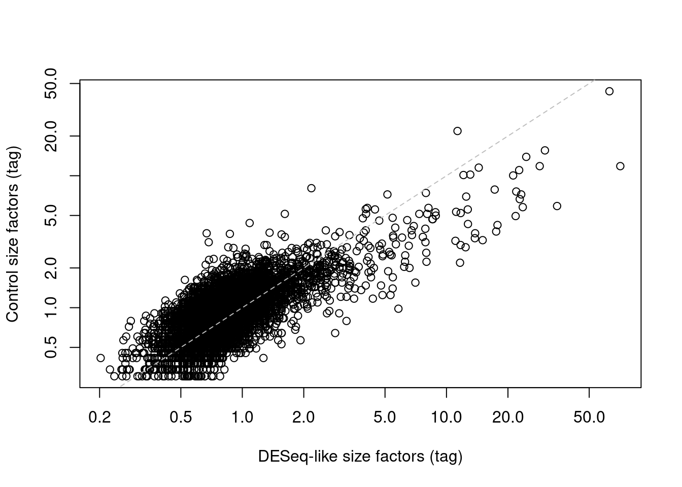
Figure 20.6: IgG control-derived size factors for each cell in the PBMC dataset, compared to the DESeq-like size factors.
This approach exchanges the previous assumption of a non-differential majority for another assumption about the lack of differential abundance in the control tags. We might feel that the latter is a generally weaker assumption, but it is possible for non-specific binding to vary due to biology (e.g., when the cell surface area increases), at which point this normalization strategy may not be appropriate. It also relies on sufficient coverage of the control ADTs, which is not always possible in well-executed experiments where there is little non-specific binding to provide such counts.
20.4.5 Computing log-normalized values
We suggest using the median-based size factors by default, as they are generally applicable and eliminate most problems with composition biases.
We set the size factors for the ADT data by calling sizeFactors() on the relevant altExp().
In contrast, sizeFactors(sce) refers to size factors for the gene counts, which are usually quite different.
Regardless of which size factors are chosen, running logNormCounts() will then perform scaling normalization and log-transformation for both the endogenous transcripts and the ADTs using their respective size factors.
sce <- logNormCounts(sce, use.altexps=TRUE)

# Checking that we have normalized values:
assayNames(sce)
## [1] "counts" "logcounts"## [1] "counts" "logcounts"20.5 Clustering and interpretation
Unlike transcript-based counts, feature selection is largely unnecessary for analyzing ADT data. This is because feature selection has already occurred during experimental design where the manual choice of target proteins means that all ADTs correspond to interesting features by definition. From a practical perspective, the ADT count matrix is already small so there is no need for data compaction from using HVGs or PCs. Moreover, each ADT is often chosen to capture some orthogonal biological signal, so there is not much extraneous noise in higher dimensions that can be readily removed. This suggests we should directly apply downstream procedures like clustering and visualization on the log-normalized abundance matrix for the ADTs (Figure 20.7).
# Set d=NA so that the function does not perform PCA.
g.adt <- buildSNNGraph(altExp(sce), d=NA)
clusters.adt <- igraph::cluster_walktrap(g.adt)$membership

# Generating a t-SNE plot.
library(scater)
set.seed(1010010)
altExp(sce) <- runTSNE(altExp(sce))
colLabels(altExp(sce)) <- factor(clusters.adt)
plotTSNE(altExp(sce), colour_by="label", text_by="label", text_col="red")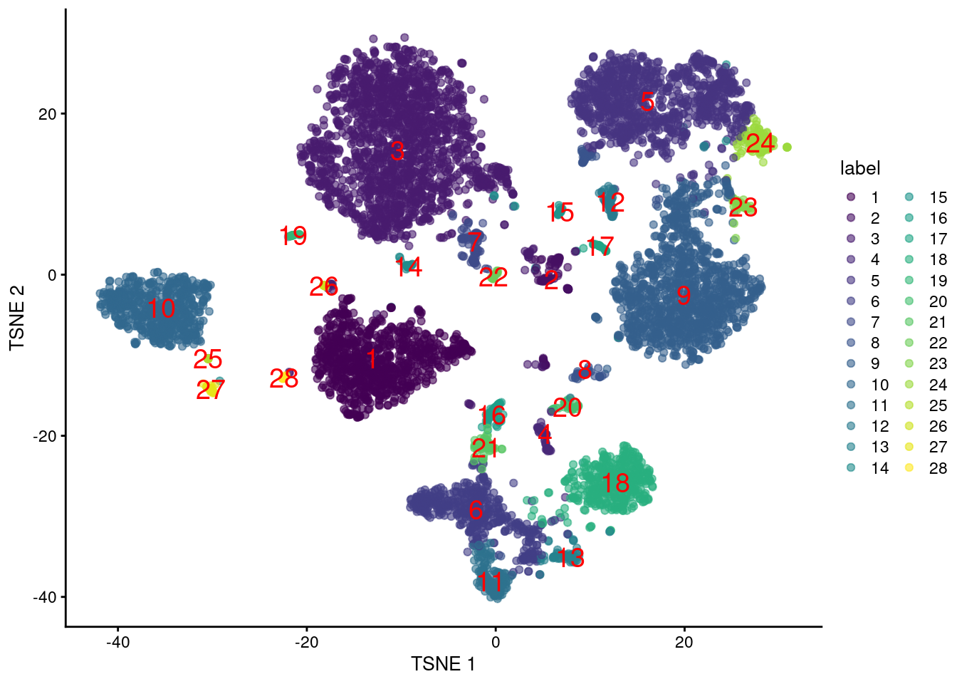
Figure 20.7: \(t\)-SNE plot generated from the log-normalized abundance of each ADT in the PBMC dataset. Each point is a cell and is labelled according to its assigned cluster.
With only a few ADTs, characterization of each cluster is most efficiently achieved by creating a heatmap of the average log-abundance of each tag (Figure 20.8).
For this experiment, we can easily identify B cells (CD19+), various subsets of T cells (CD3+, CD4+, CD8+), monocytes and macrophages (CD14+, CD16+), to name a few.
More detailed examination of the distribution of abundances within each cluster is easily performed with plotExpression() where strong bimodality may indicate that finer clustering is required to resolve cell subtypes.
se.averaged <- sumCountsAcrossCells(altExp(sce), clusters.adt,
    exprs_values="logcounts", average=TRUE)

library(pheatmap)
averaged <- assay(se.averaged)
pheatmap(averaged - rowMeans(averaged),
    breaks=seq(-3, 3, length.out=101))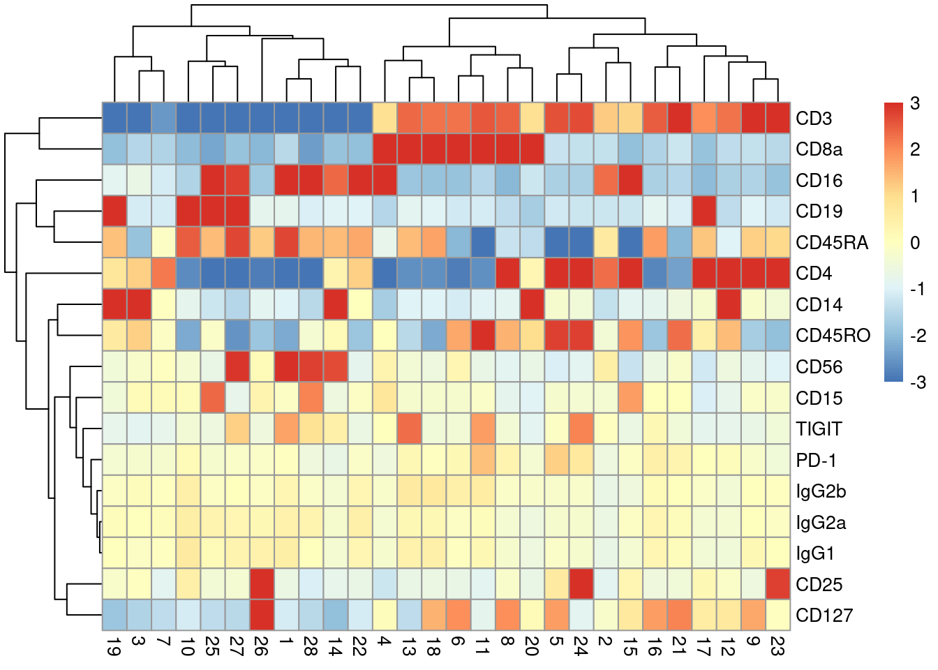
Figure 20.8: Heatmap of the average log-normalized abundance of each ADT in each cluster of the PBMC dataset. Colors represent the log2-fold change from the grand average across all clusters.
Of course, this provides little information beyond what we could have obtained from a mass cytometry experiment; the real value of this data lies in the integration of protein abundance with gene expression.
20.6 Integration with gene expression data
20.6.1 By subclustering
In the simplest approach to integration, we take cells in each of the ADT-derived clusters and perform subclustering using the transcript data.
This is an in silico equivalent to an experiment that performs FACS to isolate cell types followed by scRNA-seq for further characterization.
We exploit the fact that the ADT abundances are cleaner (larger counts, stronger signal) for more robust identification of broad cell types, and use the gene expression data to identify more subtle structure that manifests in the transcriptome.
We demonstrate below by using quickSubCluster() to loop over all of the ADT-derived clusters and subcluster on gene expression (Figure 20.9).
set.seed(101010)
all.sce <- quickSubCluster(sce, clusters.adt,
    prepFUN=function(x) {
        dec <- modelGeneVar(x)
        top <- getTopHVGs(dec, prop=0.1)
        x <- runPCA(x, subset_row=top, ncomponents=25)
    },
    clusterFUN=function(x) {
        g.trans <- buildSNNGraph(x, use.dimred="PCA")
        igraph::cluster_walktrap(g.trans)$membership
    }
)

# Summarizing the number of subclusters in each tag-derived parent cluster,
# compared to the number of cells in that parent cluster.
ncells <- vapply(all.sce, ncol, 0L)
nsubclusters <- vapply(all.sce, FUN=function(x) length(unique(x$subcluster)), 0L)
plot(ncells, nsubclusters, xlab="Number of cells", type="n",
    ylab="Number of subclusters", log="xy")
text(ncells, nsubclusters, names(all.sce))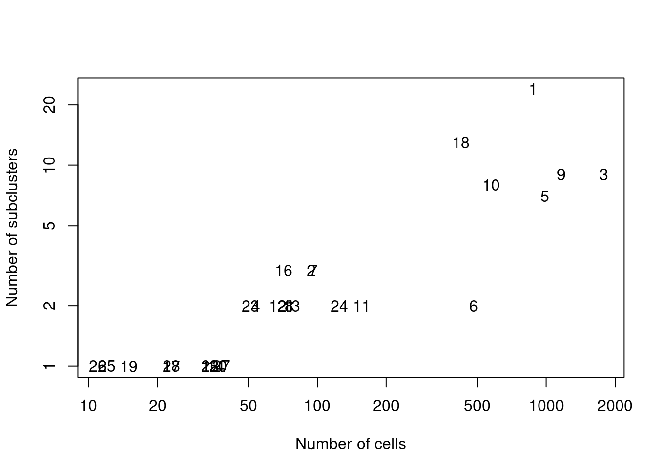
Figure 20.9: Number of subclusters identified from the gene expression data within each ADT-derived parent cluster.
Another benefit of subclustering is that we can use the annotation on the ADT-derived clusters to facilitate annotation of each subcluster.
If we knew that cluster X contained T cells from the ADT-derived data, there is no need to identify subclusters X.1, X.2, etc. as T cells from scratch; rather, we can focus on the more subtle (and interesting) differences between the subclusters using findMarkers().
For example, cluster 11 contains CD8+ T cells according to Figure 20.8, in which we further identify internal subclusters based on granzyme expression (Figure 20.10).
Subclustering is also conceptually appealing as it avoids comparing log-fold changes in protein abundances with log-fold changes in gene expression.
This ensures that variation (or noise) from the transcript counts does not compromise cell type/state identification from the relatively cleaner ADT counts.
of.interest <- "11"
plotExpression(all.sce[[of.interest]], x="subcluster",
    features=c("ENSG00000100450", "ENSG00000113088"))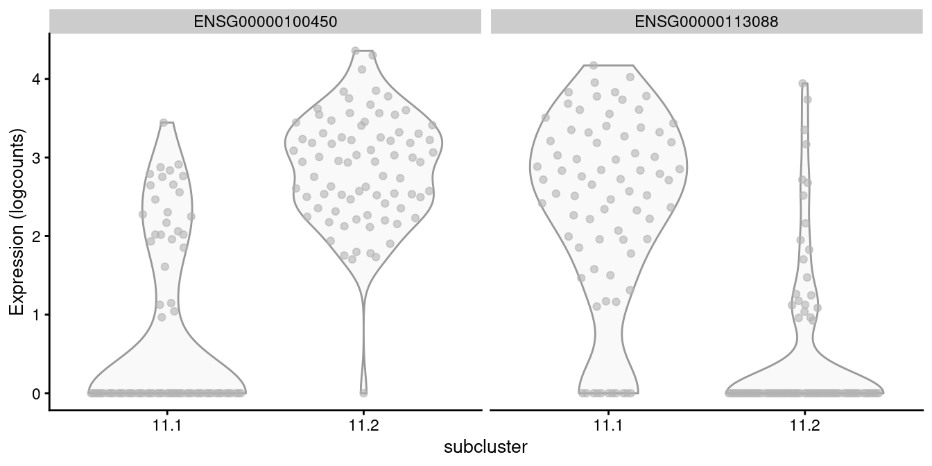
Figure 20.10: Distribution of log-normalized expression values of GZMH (left) and GZHK (right) in transcript-derived subclusters of a ADT-derived subpopulation of CD8+ T cells.
The downside is that relying on previous results increases the risk of misleading conclusions when ambiguities in those results are not considered, as previously discussed in Section 10.7. It is a good idea to perform some additional checks to ensure that each subcluster has similar protein abundances, e.g., using a heatmap as in Figure 20.8 or with a series of plots like in Figure 20.11. If so, this allows the subcluster to “inherit” the annotation attached to the parent cluster for easier interpretation.
sce.cd8 <- all.sce[[of.interest]]
plotExpression(altExp(sce.cd8), x=I(sce.cd8$subcluster),
    features=c("CD3", "CD8a"))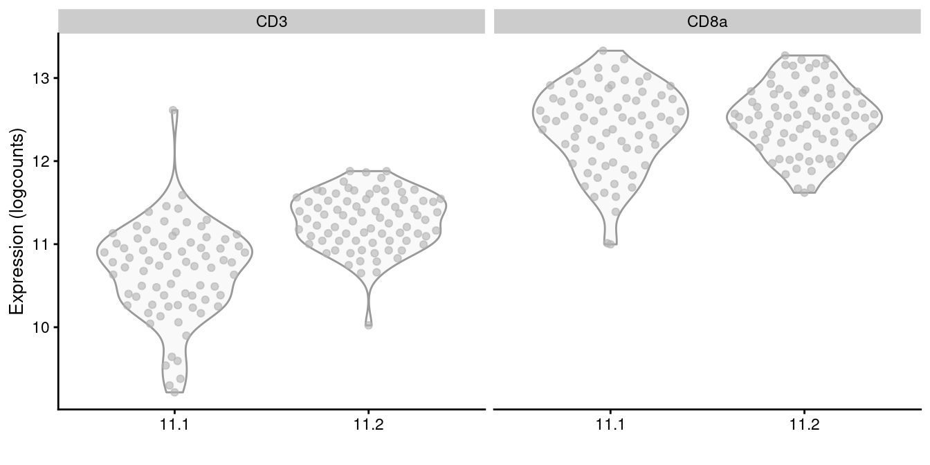
Figure 20.11: Distribution of log-normalized abundances of ADTs for CD3 and CD8a in each subcluster of the CD8+ T cell population.
20.6.2 By combined clustering
Alternatively, we can combine the information from both sets of features into a single matrix for use in downstream analyses. This is logistically convenient as the combined structure is compatible with routine analysis workflows for transcript-only data. To illustrate, we first perform some standard steps on the transcript count matrix:
sce.main <- logNormCounts(sce)
dec.main <- modelGeneVar(sce.main)
top.main <- getTopHVGs(dec.main, prop=0.1)
sce.main <- runPCA(sce.main, subset_row=top.main, ncomponents=25)
The simplest version of this idea involves literally combining the log-normalized abundance matrix for the ADTs with the log-expression matrix (or its compacted form, the matrix of PCs) to obtain a single matrix for use in downstream procedures. This requires some reweighting to balance the contribution of the transcript and ADT data to the total variance in the combined matrix, especially given that the former has around 100-fold more features than the latter. We see that the number of clusters is slightly higher than that from the ADT data alone, consistent with the introduction of additional heterogeneity when the two feature sets are combined.
# TODO: push this into a function somewhere.
library(DelayedMatrixStats)
transcript.data <- logcounts(sce.main)[top.main,,drop=FALSE]
transcript.var <- sum(rowVars(DelayedArray(transcript.data)))
tag.data <- logcounts(altExp(sce.main))
tag.var <- sum(rowVars(DelayedArray(tag.data)))

reweight <- sqrt(transcript.var/tag.var)
combined <- rbind(transcript.data, tag.data*reweight)

# 'buildSNNGraph' conveniently performs the PCA for us if requested. We use
# more PCs in 'd' to capture more variance in both sets of features. Note that
# this uses IRLBA by default so we need to set the seed.
set.seed(100010)
g.com <- buildSNNGraph(combined, d=50)
clusters.com <- igraph::cluster_walktrap(g.com)$membership
table(clusters.com)
## clusters.com
## 1 2 3 4 5 6 7 8 9 10 11 12 13 14 15 16
## 51 70 347 116 77 842 504 1121 1679 60 52 340 167 47 19 53
## 17 18 19 20 21 22 23 24 25 26 27 28 29 30 31 32
## 71 981 40 36 16 68 25 25 388 73 35 11 67 20 47 27
## 33
## 17A more sophisticated approach uses the UMAP algorithm (McInnes, Healy, and Melville 2018) to integrate information from the two sets of features. Very loosely speaking, we can imagine this as an intersection of the nearest neighbor graphs formed from each set, which effectively encourages the formation of communities of cells that are close in both feature spaces. Here, we perform two rounds of UMAP; one round retains high dimensionality for a faithful representation of the data during clustering, while the other performs dimensionality reduction for a pretty visualization. This yields an extremely fine-grained clustering in Figure 20.12, which is attributable to the stringency of intersection operations for defining the local neighborhood.
set.seed(1001010)
sce.main <- runMultiUMAP(sce.main, dimred="PCA",
    altexp="Antibody Capture", n_components=50)

# Bumping up 'k' for less granularity.
g.com2 <- buildSNNGraph(sce.main, k=20, use.dimred="MultiUMAP")
clusters.com2 <- igraph::cluster_walktrap(g.com2)$membership
table(clusters.com2)
## clusters.com2
## 1 2 3 4 5 6 7 8 9 10 11 12 13 14 15 16
## 324 173 220 704 790 123 395 733 1022 426 78 67 103 181 62 763
## 17 18 19 20 21 22 23 24 25 26 27 28 29 30 31 32
## 50 96 87 159 90 53 33 71 62 65 33 53 42 28 61 34
## 33 34 35 36 37 38 39 40 41 42
## 47 33 29 23 33 36 20 32 26 32# Combining again for visualization:
set.seed(0101110)
sce.main <- runMultiUMAP(sce.main, dimred="PCA",
altexp="Antibody Capture", name="MultiUMAP2")
colLabels(sce.main) <- clusters.com2
plotReducedDim(sce.main, "MultiUMAP2", colour_by="label", text_by="label")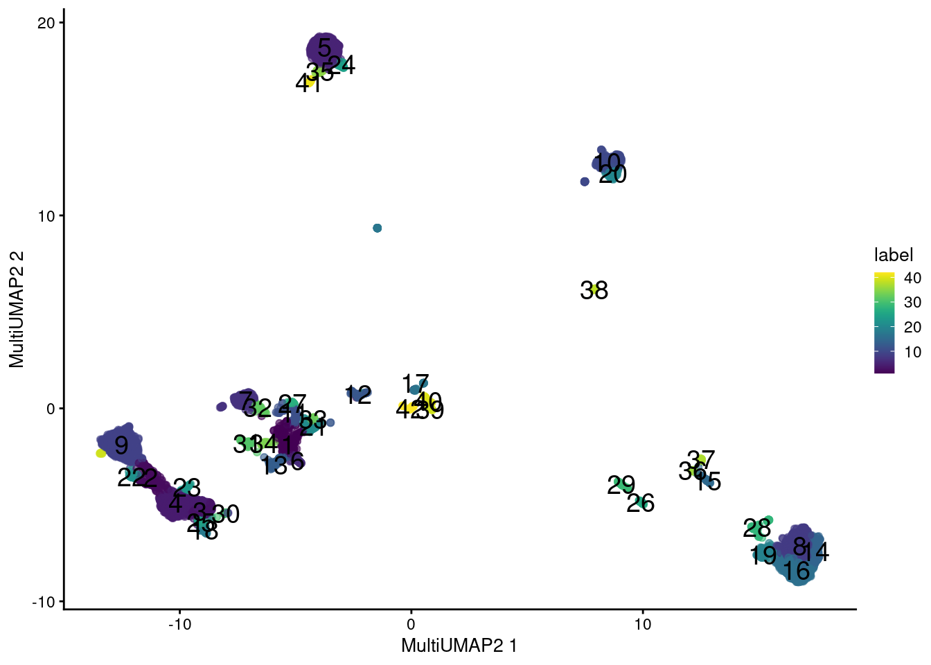
Figure 20.12: UMAP plot obtained by combining transcript and ADT data in the PBMC dataset. Each point represents a cell and is colored according to its assigned cluster.
An even more sophisticated approach uses factor analysis to identify common and unique factors of variation in each feature set. The set of factors can then be used as low-dimensional coordinates for each cell in downstream analyses, though a number of additional statistics are also computed that may be useful, e.g., the contribution of each feature to each factor.
These combined strategies are convenient but do not consider (or implicitly make assumptions about) the importance of heterogeneity in the ADT data relative to the transcript data. For example, the UMAP approach takes equal contributions from both sets of features to the intersection, which may not be appropriate if the biology of interest is concentrated in only one set. More generally, a combined analysis must consider the potential for uninteresting noise in one set to interfere with biological signal in the other set, a concern that is largely avoided during subclustering.
20.6.3 By differential testing
In more interesting applications of this technology, protein targets are chosen that reflect some functional activity rather than cell type. (Because, frankly, the latter is not particularly hard to infer from transcript data in most cases.) A particularly elegant example involves quantification of the immune response by using antibodies to target the influenza peptide-MHCII complexes in T cells, albeit for mass cytometry (Fehlings et al. 2018). If the aim is to test for differences in the functional readout, a natural analysis strategy is to use the transcript data for clustering (Figure 20.13) and perform differential testing between clusters or conditions for the relevant ADTs.
# Performing a quick analysis of the gene expression data.
sce <- logNormCounts(sce)
dec <- modelGeneVar(sce)
top <- getTopHVGs(dec, prop=0.1)

set.seed(1001010)
sce <- runPCA(sce, subset_row=top, ncomponents=25)

g <- buildSNNGraph(sce, use.dimred="PCA")
clusters <- igraph::cluster_walktrap(g)$membership
colLabels(sce) <- factor(clusters)

set.seed(1000010)
sce <- runTSNE(sce, dimred="PCA")
plotTSNE(sce, colour_by="label", text_by="label")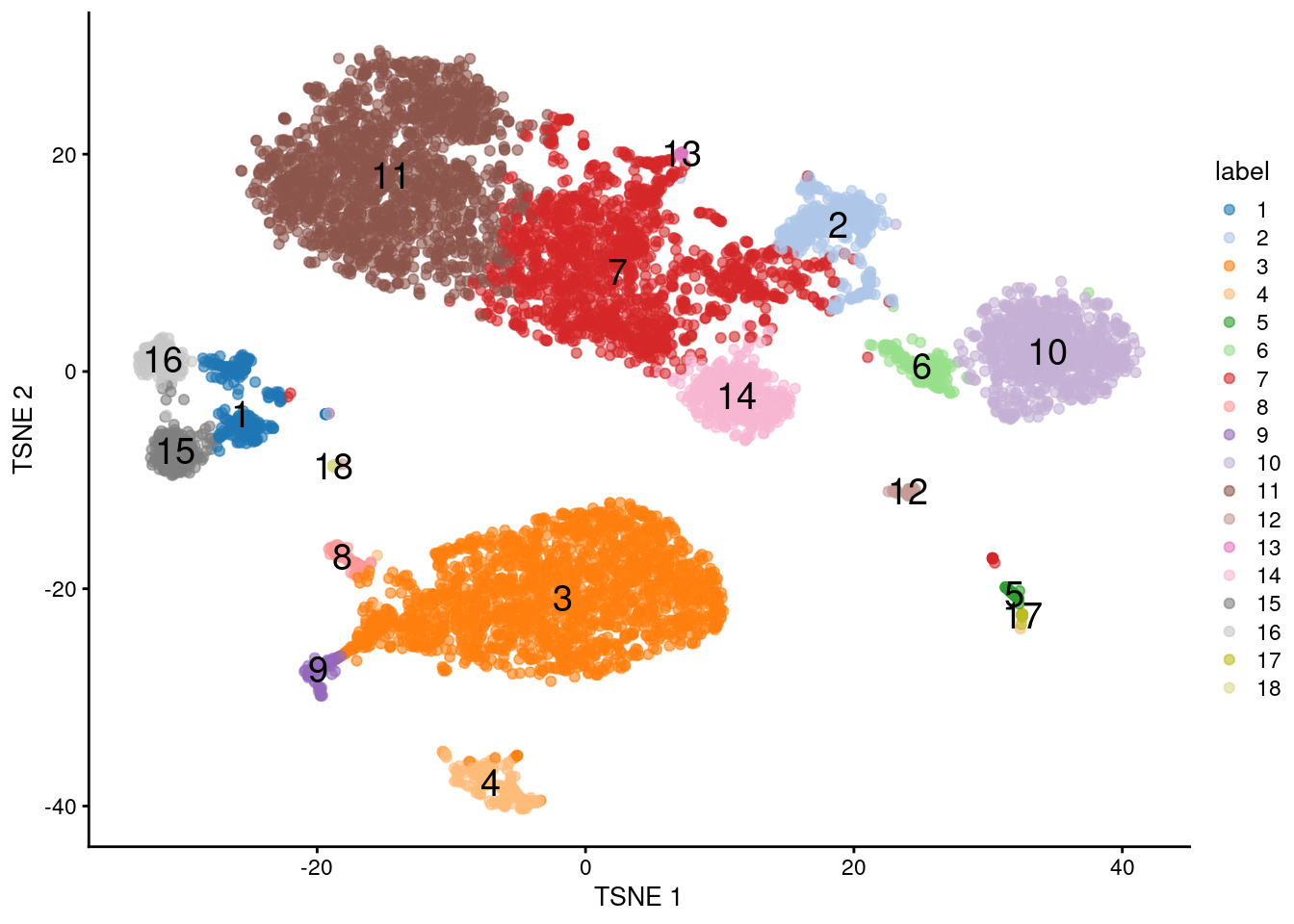
Figure 20.13: \(t\)-SNE plot of the PBMC dataset based on the transcript data. Each point is a cell and is colored according to the assigned cluster.
We demonstrate this approach using findMarkers() to test for differences in tag abundance between clusters (Chapter 11).
For example, if the PD-1 level was a readout for some interesting phenotype - say, T cell exhaustion (Pauken and Wherry 2015) - we might be interested in its upregulation in cluster 13 compared to all other clustuers (Figure 20.14).
Methods from Chapter 14 can be similarly used to test for differences between conditions based on pseudo-bulk ADT counts.
markers <- findMarkers(altExp(sce), colLabels(sce))
of.interest <- markers[[13]]
pheatmap(getMarkerEffects(of.interest), breaks=seq(-3, 3, length.out=101))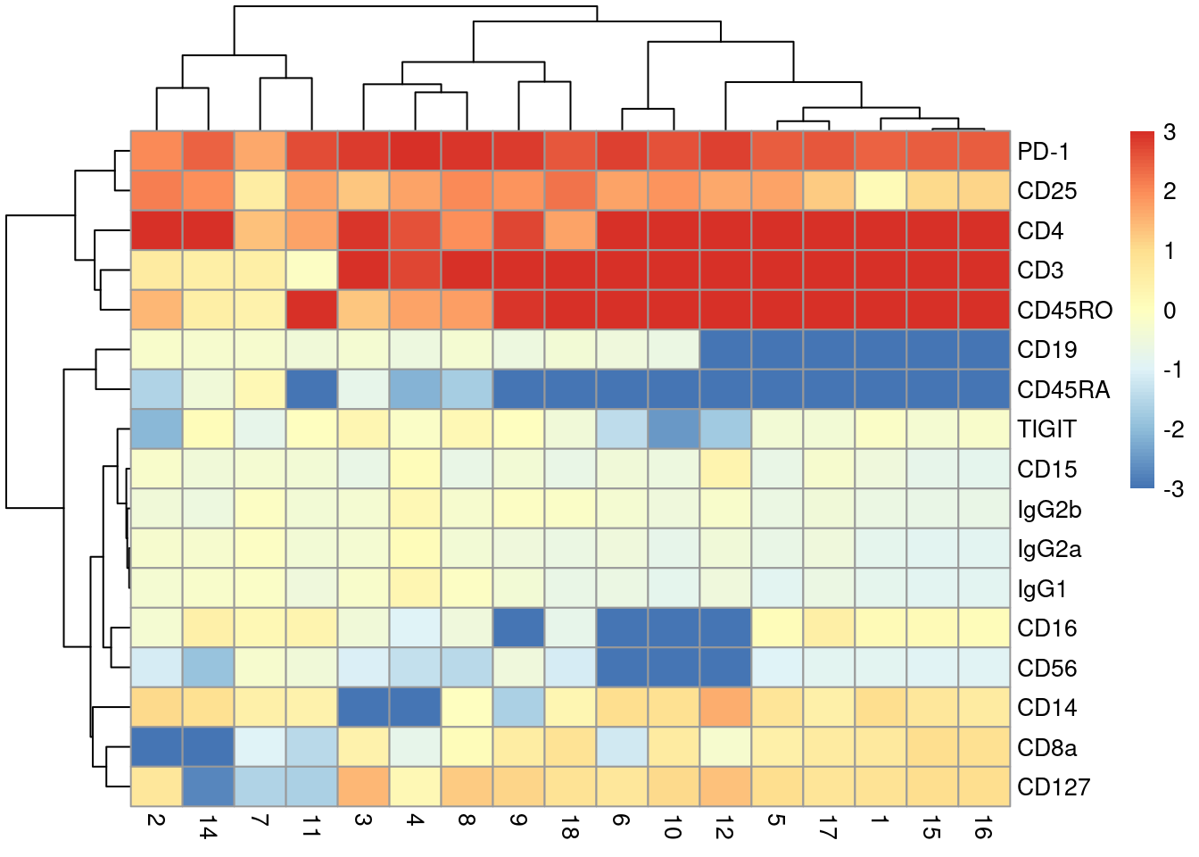
Figure 20.14: Heatmap of log-fold changes in tag abundances in cluster 13 compared to all other clusters identified from transcript data in the PBMC data set.
The main appeal of this approach is that it avoids data snooping (Section 11.5.1) as the clusters are defined without knowledge of the ADTs. This improves the statistical rigor of the subsequent differential testing on the ADT abundances (though only to some extent; other problems are still present, such as the lack of true replication in between-cluster comparisons). From a practical perspective, this approach yields fewer clusters and reduces the amount of work involved in manual annotation, especially if there are multiple functional states (e.g., stressed, apoptotic, stimulated) for each cell type. However, it is fundamentally limited to per-tag inferences; if we want to identify subpopulations with interesting combinations of target proteins, we must resort to high-dimensional analyses like clustering on the ADT abundances.
Session Info
R version 4.0.4 (2021-02-15)
Platform: x86_64-pc-linux-gnu (64-bit)
Running under: Ubuntu 20.04.2 LTS

Matrix products: default
BLAS:   /home/biocbuild/bbs-3.12-books/R/lib/libRblas.so
LAPACK: /home/biocbuild/bbs-3.12-books/R/lib/libRlapack.so

locale:
 [1] LC_CTYPE=en_US.UTF-8       LC_NUMERIC=C
 [3] LC_TIME=en_US.UTF-8        LC_COLLATE=C
 [5] LC_MONETARY=en_US.UTF-8    LC_MESSAGES=en_US.UTF-8
 [7] LC_PAPER=en_US.UTF-8       LC_NAME=C
 [9] LC_ADDRESS=C               LC_TELEPHONE=C
[11] LC_MEASUREMENT=en_US.UTF-8 LC_IDENTIFICATION=C

attached base packages:
[1] parallel  stats4    stats     graphics  grDevices utils     datasets
[8] methods   base

other attached packages:
 [1] DelayedMatrixStats_1.12.3   DelayedArray_0.16.2
 [3] Matrix_1.3-2                pheatmap_1.0.12
 [5] scran_1.18.5                scater_1.18.6
 [7] ggplot2_3.3.3               scuttle_1.0.4
 [9] DropletUtils_1.10.3         SingleCellExperiment_1.12.0
[11] SummarizedExperiment_1.20.0 Biobase_2.50.0
[13] GenomicRanges_1.42.0        GenomeInfoDb_1.26.4
[15] IRanges_2.24.1              S4Vectors_0.28.1
[17] BiocGenerics_0.36.0         MatrixGenerics_1.2.1
[19] matrixStats_0.58.0          DropletTestFiles_1.0.0
[21] BiocStyle_2.18.1            rebook_1.0.0

loaded via a namespace (and not attached):
  [1] AnnotationHub_2.22.0          BiocFileCache_1.14.0
  [3] igraph_1.2.6                  BiocParallel_1.24.1
  [5] digest_0.6.27                 htmltools_0.5.1.1
  [7] viridis_0.5.1                 fansi_0.4.2
  [9] magrittr_2.0.1                memoise_2.0.0
 [11] limma_3.46.0                  R.utils_2.10.1
 [13] colorspace_2.0-0              blob_1.2.1
 [15] rappdirs_0.3.3                xfun_0.22
 [17] dplyr_1.0.5                   callr_3.5.1
 [19] crayon_1.4.1                  RCurl_1.98-1.3
 [21] jsonlite_1.7.2                graph_1.68.0
 [23] glue_1.4.2                    gtable_0.3.0
 [25] zlibbioc_1.36.0               XVector_0.30.0
 [27] BiocSingular_1.6.0            Rhdf5lib_1.12.1
 [29] HDF5Array_1.18.1              scales_1.1.1
 [31] DBI_1.1.1                     edgeR_3.32.1
 [33] Rcpp_1.0.6                    viridisLite_0.3.0
 [35] xtable_1.8-4                  dqrng_0.2.1
 [37] bit_4.0.4                     rsvd_1.0.3
 [39] httr_1.4.2                    RColorBrewer_1.1-2
 [41] ellipsis_0.3.1                pkgconfig_2.0.3
 [43] XML_3.99-0.6                  R.methodsS3_1.8.1
 [45] farver_2.1.0                  uwot_0.1.10
 [47] CodeDepends_0.6.5             sass_0.3.1
 [49] dbplyr_2.1.0                  locfit_1.5-9.4
 [51] utf8_1.2.1                    tidyselect_1.1.0
 [53] labeling_0.4.2                rlang_0.4.10
 [55] later_1.1.0.1                 AnnotationDbi_1.52.0
 [57] munsell_0.5.0                 BiocVersion_3.12.0
 [59] tools_4.0.4                   cachem_1.0.4
 [61] generics_0.1.0                RSQLite_2.2.4
 [63] ExperimentHub_1.16.0          evaluate_0.14
 [65] stringr_1.4.0                 fastmap_1.1.0
 [67] yaml_2.2.1                    processx_3.4.5
 [69] knitr_1.31                    bit64_4.0.5
 [71] purrr_0.3.4                   sparseMatrixStats_1.2.1
 [73] mime_0.10                     R.oo_1.24.0
 [75] compiler_4.0.4                beeswarm_0.3.1
 [77] curl_4.3                      interactiveDisplayBase_1.28.0
 [79] tibble_3.1.0                  statmod_1.4.35
 [81] bslib_0.2.4                   stringi_1.5.3
 [83] highr_0.8                     ps_1.6.0
 [85] RSpectra_0.16-0               lattice_0.20-41
 [87] bluster_1.0.0                 vctrs_0.3.6
 [89] pillar_1.5.1                  lifecycle_1.0.0
 [91] rhdf5filters_1.2.0            BiocManager_1.30.10
 [93] jquerylib_0.1.3               RcppAnnoy_0.0.18
 [95] BiocNeighbors_1.8.2           cowplot_1.1.1
 [97] bitops_1.0-6                  irlba_2.3.3
 [99] httpuv_1.5.5                  R6_2.5.0
[101] bookdown_0.21                 promises_1.2.0.1
[103] gridExtra_2.3                 vipor_0.4.5
[105] codetools_0.2-18              assertthat_0.2.1
[107] rhdf5_2.34.0                  withr_2.4.1
[109] GenomeInfoDbData_1.2.4        grid_4.0.4
[111] beachmat_2.6.4                rmarkdown_2.7
[113] Rtsne_0.15                    shiny_1.6.0
[115] ggbeeswarm_0.6.0
Bibliography
Fehlings, M., S. Chakarov, Y. Simoni, B. Sivasankar, F. Ginhoux, and E. W. Newell. 2018. “Multiplex peptide-MHC tetramer staining using mass cytometry for deep analysis of the influenza-specific T-cell response in mice.” J. Immunol. Methods 453 (February): 30–36.
McInnes, Leland, John Healy, and James Melville. 2018. “UMAP: Uniform Manifold Approximation and Projection for Dimension Reduction.” arXiv E-Prints, February, arXiv:1802.03426. http://arxiv.org/abs/1802.03426.
Pauken, K. E., and E. J. Wherry. 2015. “Overcoming T cell exhaustion in infection and cancer.” Trends Immunol. 36 (4): 265–76.
Stoeckius, M., C. Hafemeister, W. Stephenson, B. Houck-Loomis, P. K. Chattopadhyay, H. Swerdlow, R. Satija, and P. Smibert. 2017. “Simultaneous epitope and transcriptome measurement in single cells.” Nat. Methods 14 (9): 865–68.
Zheng, G. X., J. M. Terry, P. Belgrader, P. Ryvkin, Z. W. Bent, R. Wilson, S. B. Ziraldo, et al. 2017. “Massively parallel digital transcriptional profiling of single cells.” Nat Commun 8 (January): 14049.