Chapter 4 Data Infrastructure
4.1 Background
One of the main strengths of the Bioconductor project lies in the use of a common data infrastructure that powers interoperability across packages.
Users should be able to analyze their data using functions from different Bioconductor packages without the need to convert between formats.
To this end, the SingleCellExperiment class (from the SingleCellExperiment package) serves as the common currency for data exchange across 70+ single-cell-related Bioconductor packages.
This class implements a data structure that stores all aspects of our single-cell data - gene-by-cell expression data, per-cell metadata and per-gene annotation (Figure 4.1) - and manipulate them in a synchronized manner.
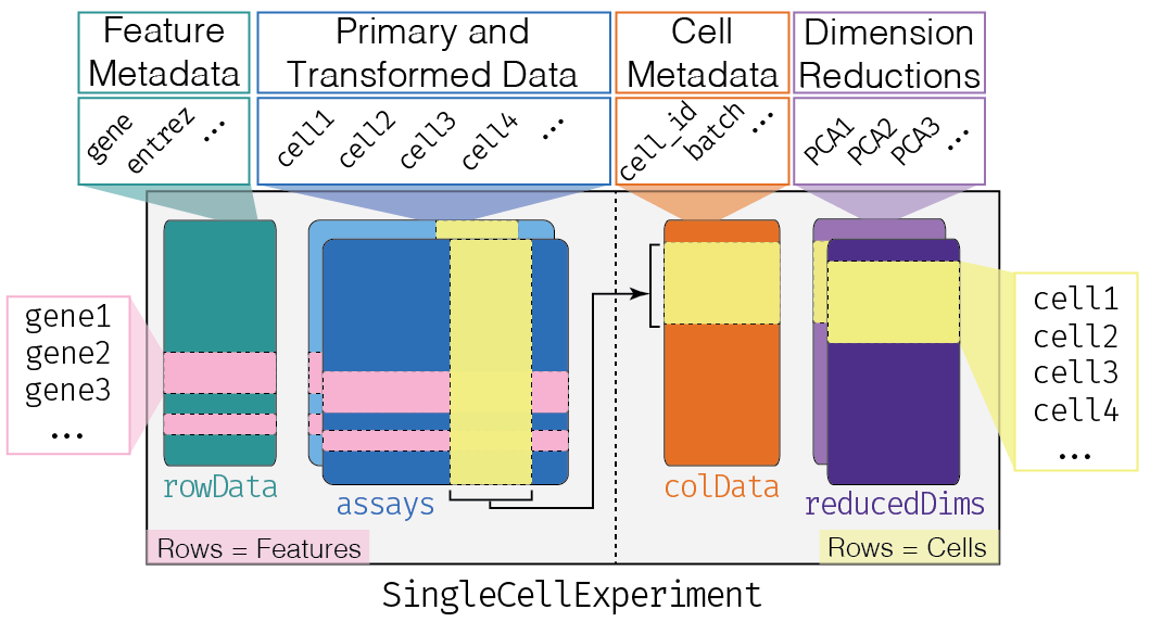
Figure 4.1: Overview of the structure of the SingleCellExperiment class. Each row of the assays corresponds to a row of the rowData (pink shading), while each column of the assays corresponds to a column of the colData and reducedDims (yellow shading).
The SingleCellExperiment package is implicitly installed and loaded when using any package that depends on the SingleCellExperiment class, but it can also be explicitly installed (and loaded) as follows:
Additionally, we use some functions from the scater and scran packages, as well as the CRAN package uwot (which conveniently can also be installed through BiocManager::install).
These functions will be accessed through the <package>::<function> convention as needed.
We then load the SingleCellExperiment package into our R session.
This avoids the need to prefix our function calls with ::, especially for packages that are heavily used throughout a workflow.
Each piece of (meta)data in the SingleCellExperiment is represented by a separate “slot”.
(This terminology comes from the S4 class system, but that’s not important right now.)
If we imagine the SingleCellExperiment object to be a cargo ship, the slots can be thought of as individual cargo boxes with different contents, e.g., certain slots expect numeric matrices whereas others may expect data frames.
In the rest of this chapter, we will discuss the available slots, their expected formats, and how we can interact with them.
More experienced readers may note the similarity with the SummarizedExperiment class, and if you are such a reader, you may wish to jump directly to the end of this chapter for the single-cell-specific aspects of this class.
4.2 Storing primary experimental data
4.2.1 Filling the assays slot
To construct a rudimentary SingleCellExperiment object, we only need to fill the assays slot.
This contains primary data such as a matrix of sequencing counts where rows correspond to features (genes) and columns correspond to samples (cells) (Figure 4.1, blue box).
Let’s start simple by generating three cells’ worth of count data across ten genes:
counts_matrix <- data.frame(cell_1 = rpois(10, 10),
                    cell_2 = rpois(10, 10),
                    cell_3 = rpois(10, 30))
rownames(counts_matrix) <- paste0("gene_", 1:10)
counts_matrix <- as.matrix(counts_matrix) # must be a matrix object!
From this, we can now construct our first SingleCellExperiment object using the SingleCellExperiment() function.
Note that we provide our data as a named list where each entry of the list is a matrix.
Here, we name the counts_matrix entry as simply "counts".
To inspect the object, we can simply type sce into the console to see some pertinent information, which will display an overview of the various slots available to us (which may or may not have any data).
## class: SingleCellExperiment
## dim: 10 3
## metadata(0):
## assays(1): counts
## rownames(10): gene_1 gene_2 ... gene_9 gene_10
## rowData names(0):
## colnames(3): cell_1 cell_2 cell_3
## colData names(0):
## reducedDimNames(0):
## altExpNames(0):
To access the count data we just supplied, we can do any one of the following:
assay(sce, "counts")- this is the most general method, where we can supply the name of the assay as the second argument.counts(sce)- this is a short-cut for the above, but only works for assays with the special name"counts".
##         cell_1 cell_2 cell_3
## gene_1       8     16     25
## gene_2       9     13     30
## gene_3       9     13     27
## gene_4      12      8     35
## gene_5      12     12     27
## gene_6      14     11     32
## gene_7      11      8     34
## gene_8       6     11     30
## gene_9       6     18     26
## gene_10      7     13     23
4.2.2 Adding more assays
What makes the assays slot especially powerful is that it can hold multiple representations of the primary data.
This is especially useful for storing the raw count matrix as well as a normalized version of the data.
We can do just that as shown below, using the scater package to compute a normalized and log-transformed representation of the initial primary data.
Note that, at each step, we overwrite our previous sce by reassigning the results back to sce.
This is possible because these particular functions return a SingleCellExperiment object that contains the results in addition to original data.
(Some functions - especially those outside of single-cell oriented Bioconductor packages - do not, in which case you will need to append your results to the sce object - see below for an example.)
Viewing the object again, we see that these functions added some new entries:
## class: SingleCellExperiment
## dim: 10 3
## metadata(0):
## assays(2): counts logcounts
## rownames(10): gene_1 gene_2 ... gene_9 gene_10
## rowData names(0):
## colnames(3): cell_1 cell_2 cell_3
## colData names(1): sizeFactor
## reducedDimNames(0):
## altExpNames(0):
Specifically, we see that the assays slot has grown to contain two entries: "counts" (our initial data) and "logcounts" (the log-transformed normalized data).
Similar to "counts", the "logcounts" name can be conveniently accessed using logcounts(sce), although the longhand version works just as well.
##           cell_1   cell_2   cell_3
## gene_1  3.940600 4.519817 3.962599
## gene_2  4.100047 4.234697 4.210128
## gene_3  4.100047 4.234697 4.066760
## gene_4  4.493898 3.581374 4.421342
## gene_5  4.493898 4.125592 4.066760
## gene_6  4.707114 4.007555 4.298357
## gene_7  4.374176 3.581374 4.381501
## gene_8  3.556547 4.007555 4.210128
## gene_9  3.556547 4.682738 4.015619
## gene_10 3.761315 4.234697 3.850329
To look at all the available assays within sce, we can use the assays() accessor.
By comparison, assay() only returns a single assay of interest.
## List of length 2
## names(2): counts logcounts
While the functions above automatically add assays to our sce object, there may be cases where we want to perform our own calculations and save the result into the assays slot.
This is often necessary when using functions that do not return a SingleCellExperiment object.
To illustrate, let’s append a new version of the data that has been offset by adding 100 to all values.
counts_100 <- counts(sce) + 100
assay(sce, "counts_100") <- counts_100 # assign a new entry to assays slot
assays(sce) # new assay has now been added.
## List of length 3
## names(3): counts logcounts counts_1004.3 Handling metadata
4.3.1 On the columns
To further annotate our SingleCellExperiment object, we can add metadata to describe the columns of our primary data, e.g., the samples or cells of our experiment.
This data is entered into the colData slot, a data.frame or DataFrame object where rows correspond to cells and columns correspond to metadata fields, e.g., batch of origin, treatment condition (Figure 4.1, orange box).
Let’s come up with some metadata for the cells, starting with a batch variable where cells 1 and 2 are in batch 1 and cell 3 is from batch 2.
Now, we can take two approaches - either append the cell_metadata to our existing sce, or start from scratch via the SingleCellExperiment() constructor.
We’ll start from scratch for now:
Similar to assays, we can see our colData is now populated:
## class: SingleCellExperiment
## dim: 10 3
## metadata(0):
## assays(1): counts
## rownames(10): gene_1 gene_2 ... gene_9 gene_10
## rowData names(0):
## colnames(3): cell_1 cell_2 cell_3
## colData names(1): batch
## reducedDimNames(0):
## altExpNames(0):
We can access our column data with the colData() function:
## DataFrame with 3 rows and 1 column
##            batch
##        <numeric>
## cell_1         1
## cell_2         1
## cell_3         2
Or even more simply, we can extract a single field using the $ shortcut:
## [1] 1 1 2Some functions automatically add column metadata by returning a SingleCellExperiment with extra fields in the colData slot.
For example, the scater package contains the addPerCellQC() function that appends a lot of quality control data.
Here, we show the first five columns of colData(sce) with the quality control metrics appended to it.
## DataFrame with 3 rows and 4 columns
##            batch       sum  detected     total
##        <numeric> <numeric> <numeric> <numeric>
## cell_1         1        94        10        94
## cell_2         1       123        10       123
## cell_3         2       289        10       289
Alternatively, we might want to manually add more fields to the column metadata:
## [1] "batch" "sum" "detected" "total" "more_stuff"A common operation with colData is to use its values for subsetting.
For example, if we only wanted cells within batch 1, we could subset our sce object as shown below.
(Remember, we subset on the columns in this case because we are filtering by cells/samples here.)
## class: SingleCellExperiment
## dim: 10 2
## metadata(0):
## assays(1): counts
## rownames(10): gene_1 gene_2 ... gene_9 gene_10
## rowData names(0):
## colnames(2): cell_1 cell_2
## colData names(5): batch sum detected total more_stuff
## reducedDimNames(0):
## altExpNames(0):
4.3.2 On the rows
To store feature-level annotation, the SingleCellExperiment has the rowData slot containing a DataFrame where each row corresponds to a gene and contains annotations like the transcript length or gene symbol.
Furthermore, there is a special rowRanges slot to hold genomic coordinates in the form of a GRanges or GRangesList.
This stores describes the chromosome, start, and end coordinates of the features (genes, genomic regions) in a manner that is easy to query and manipulate via the GenomicRanges framework.
Both of these slots can be accessed via their respective accessors, rowRanges() and rowData().
In our case, rowRanges(sce) produces an empty list because we did not fill it with any coordinate information.
## GRangesList object of length 10:
## $gene_1
## GRanges object with 0 ranges and 0 metadata columns:
##    seqnames    ranges strand
##       <Rle> <IRanges>  <Rle>
##   -------
##   seqinfo: no sequences
##
## $gene_2
## GRanges object with 0 ranges and 0 metadata columns:
##    seqnames    ranges strand
##       <Rle> <IRanges>  <Rle>
##   -------
##   seqinfo: no sequences
##
## $gene_3
## GRanges object with 0 ranges and 0 metadata columns:
##    seqnames    ranges strand
##       <Rle> <IRanges>  <Rle>
##   -------
##   seqinfo: no sequences
##
## ...
## <7 more elements>
Currently the rowData slot is also empty.
However, analogous to our call to addPerCellQC() in the prior section, the addPerFeatureQC() function will insert values in the rowData slot of our sce object:
## DataFrame with 10 rows and 2 columns
##              mean  detected
##         <numeric> <numeric>
## gene_1    16.3333       100
## gene_2    17.3333       100
## gene_3    16.3333       100
## gene_4    18.3333       100
## gene_5    17.0000       100
## gene_6    19.0000       100
## gene_7    17.6667       100
## gene_8    15.6667       100
## gene_9    16.6667       100
## gene_10   14.3333       100
In a similar fashion to the colData slot, such feature metadata could be provided at the onset when creating the SingleCellExperiment object.
Exactly how this is done depends on the organism and annotation available during alignment and quantification;
for example, given Ensembl identifiers, we might use AnnotationHub resources to pull down an Ensembl anotation object and extract the gene bodies to store in the rowRanges of our SingleCellExperiment.
## GRanges object with 67667 ranges and 1 metadata column:
##                   seqnames            ranges strand |   gene_name
##                      <Rle>         <IRanges>  <Rle> | <character>
##   ENSG00000223972        1       11869-14409      + |     DDX11L1
##   ENSG00000227232        1       14404-29570      - |      WASH7P
##   ENSG00000278267        1       17369-17436      - |   MIR6859-1
##   ENSG00000243485        1       29554-31109      + | MIR1302-2HG
##   ENSG00000284332        1       30366-30503      + |   MIR1302-2
##               ...      ...               ...    ... .         ...
##   ENSG00000224240        Y 26549425-26549743      + |     CYCSP49
##   ENSG00000227629        Y 26586642-26591601      - |  SLC25A15P1
##   ENSG00000237917        Y 26594851-26634652      - |     PARP4P1
##   ENSG00000231514        Y 26626520-26627159      - |      CCNQP2
##   ENSG00000235857        Y 56855244-56855488      + |     CTBP2P1
##   -------
##   seqinfo: 424 sequences from GRCh38 genome
To subset a SingleCellExperiment object at the feature/gene level, we can do a row subsetting operation similar to other R objects, by supplying either numeric indices or a vector of names:
## class: SingleCellExperiment
## dim: 2 3
## metadata(0):
## assays(1): counts
## rownames(2): gene_1 gene_4
## rowData names(2): mean detected
## colnames(3): cell_1 cell_2 cell_3
## colData names(5): batch sum detected total more_stuff
## reducedDimNames(0):
## altExpNames(0):## class: SingleCellExperiment
## dim: 2 3
## metadata(0):
## assays(1): counts
## rownames(2): gene_1 gene_4
## rowData names(2): mean detected
## colnames(3): cell_1 cell_2 cell_3
## colData names(5): batch sum detected total more_stuff
## reducedDimNames(0):
## altExpNames(0):4.3.3 Other metadata
Some analyses contain results or annotations that do not fit into the aforementioned slots, e.g., study metadata.
Thankfully, there is a slot just for this type of messy data - the metadata slot, a named list of entries where each entry in the list can be anything you want it to be.
For example, say we have some favorite genes (e.g., highly variable genes) that we want to store inside of sce for use in our analysis at a later point.
We can do this simply by appending to the metadata slot as follows:
## $favorite_genes
## [1] "gene_1" "gene_5"
Similarly, we can append more information via the $ operator:
## $favorite_genes
## [1] "gene_1" "gene_5"
##
## $your_genes
## [1] "gene_4" "gene_8"
4.4 Single-cell-specific fields
4.4.1 Background
So far, we have covered the assays (primary data), colData (cell metadata), rowData/rowRanges (feature metadata), and metadata slots (other) of the SingleCellExperiment class.
These slots are actually inherited from the SummarizedExperiment parent class (see here for details), so any method that works on a SummarizedExperiment will also work on a SingleCellExperiment object.
But why do we need a separate SingleCellExperiment class?
This is motivated by the desire to streamline some single-cell-specific operations, which we will discuss in the rest of this section.
4.4.2 Dimensionality reduction results
The reducedDims slot is specially designed to store reduced dimensionality representations of the primary data obtained by methods such as PCA and \(t\)-SNE (see Chapter 9 for more details).
This slot contains a list of numeric matrices of low-reduced representations of the primary data, where the rows represent the columns of the primary data (i.e., cells), and columns represent the dimensions.
As this slot holds a list, we can store multiple PCA/\(t\)-SNE/etc. results for the same dataset.
In our example, we can calculate a PCA representation of our data using the runPCA() function from scater.
We see that the sce now shows a new reducedDim that can be retrieved with the accessor reducedDim().
##               PC1        PC2
## cell_1 -0.8778588 -0.3323026
## cell_2  1.1512369 -0.1409999
## cell_3 -0.2733781  0.4733024
## attr(,"varExplained")
## [1] 1.0853591 0.1771606
## attr(,"percentVar")
## [1] 85.9677 14.0323
## attr(,"rotation")
##                 PC1         PC2
## gene_9   0.53945842  0.16506870
## gene_4  -0.47481793  0.26621235
## gene_7  -0.42138376  0.32527437
## gene_6  -0.31953155 -0.26763287
## gene_8   0.15688029  0.69357794
## gene_1   0.30441645 -0.20110929
## gene_10  0.23984703 -0.06947464
## gene_5  -0.14153714 -0.42400672
## gene_3   0.07560372 -0.09804875
## gene_2   0.05754807  0.09346258
We can also calculate a tSNE representation using the scater package function runTSNE():
## Perplexity should be lower than K!## [,1] [,2]
## cell_1 -5077.5985 -2558.224
## cell_2 4761.2737 -3124.250
## cell_3 316.3247 5682.474We can view the names of all our entries in the reducedDims slot via the accessor, reducedDims().
Note that this is plural and returns a list of all results, whereas reducedDim() only returns a single result.
## List of length 2
## names(2): PCA TSNE
We can also manually add content to the reducedDims() slot, much like how we added matrices to the assays slot previously.
To illustrate, we run the umap() function directly from the uwot package to generate a matrix of UMAP coordinates that is added to the reducedDims of our sce object.
(In practice, scater has a runUMAP() wrapper function that adds the results for us, but we will manually call umap() here for demonstration purposes.)
u <- uwot::umap(t(logcounts(sce)), n_neighbors = 2)
reducedDim(sce, "UMAP_uwot") <- u
reducedDims(sce) # Now stored in the object.
## List of length 3
## names(3): PCA TSNE UMAP_uwot## [,1] [,2]
## cell_1 -0.762756 -0.7608464
## cell_2 0.140951 0.1457694
## cell_3 0.621805 0.6150770
## attr(,"scaled:center")
## [1] -5.317163 3.3906214.4.3 Alternative Experiments
The SingleCellExperiment class provides the concept of “alternative Experiments” where we have data for a distinct set of features but the same set of samples/cells.
The classic application would be to store the per-cell counts for spike-in transcripts; this allows us to retain this data for downstream use but separate it from the assays holding the counts for endogenous genes.
The separation is particularly important as such alternative features often need to be processed separately, see Chapter 20 for examples on antibody-derived tags.
If we have data for alternative feature sets, we can store it in our SingleCellExperiment as an alternative Experiment.
For example, if we have some data for spike-in transcripts, we first create a separate SummarizedExperiment object:
spike_counts <- cbind(cell_1 = rpois(5, 10),
    cell_2 = rpois(5, 10),
    cell_3 = rpois(5, 30))
rownames(spike_counts) <- paste0("spike_", 1:5)
spike_se <- SummarizedExperiment(list(counts=spike_counts))
spike_se
## class: SummarizedExperiment
## dim: 5 3
## metadata(0):
## assays(1): counts
## rownames(5): spike_1 spike_2 spike_3 spike_4 spike_5
## rowData names(0):
## colnames(3): cell_1 cell_2 cell_3
## colData names(0):Then we store this SummarizedExperiment in our sce object via the altExp() setter.
Like assays() and reducedDims(), we can also retrieve all of the available alternative Experiments with altExps().
## List of length 1
## names(1): spike
The alternative Experiment concept ensures that all relevant aspects of a single-cell dataset can be held in a single object.
It is also convenient as it ensures that our spike-in data is synchronized with the data for the endogenous genes.
For example, if we subsetted sce, the spike-in data would be subsetted to match:
## class: SummarizedExperiment
## dim: 5 2
## metadata(0):
## assays(1): counts
## rownames(5): spike_1 spike_2 spike_3 spike_4 spike_5
## rowData names(0):
## colnames(2): cell_1 cell_2
## colData names(0):
Any SummarizedExperiment object can be stored as an alternative Experiment, including another SingleCellExperiment!
This allows power users to perform tricks like those described in Section 8.5.
4.4.4 Size factors
The sizeFactors() function allows us to get or set a numeric vector of per-cell scaling factors used for normalization (see Chapter 7 for more details).
This is typically automatically added by normalization functions, as shown below for scran’s deconvolution-based size factors:
## [1] 0.5573123 0.7292490 1.7134387Alternatively, we can manually add the size factors, as shown below for library size-derived factors:
##    cell_1    cell_2    cell_3
## 0.5573123 0.7292490 1.7134387
Technically speaking, the sizeFactors concept is not unique to single-cell analyses.
Nonetheless, we mention it here as it is an extension beyond what is available in the SummarizedExperiment parent class.
4.4.5 Column labels
The colLabels() function allows us to get or set a vector or factor of per-cell labels,
typically corresponding to groupings assigned by unsupervised clustering (see Chapter 10)
or predicted cell type identities from classification algorithms (Chapter 12).
## [1] "A" "B" "C"This is a convenient field to set as several functions (e.g., scran::findMarkers) will attempt to automatically retrieve the labels via colLabels().
We can thus avoid the few extra keystrokes that would otherwise be necessary to specify, say, the cluster assignments in the function call.
4.5 Conclusion
The widespread use of the SingleCellExperiment class provides the foundation for interoperability between single-cell-related packages in the Bioconductor ecosystem.
SingleCellExperiment objects generated by one package can be used as input into another package, encouraging synergies that enable our analysis to be greater than the sum of its parts.
Each step of the analysis will also add new entries to the assays, colData, reducedDims, etc.,
meaning that the final SingleCellExperiment object effectively serves as a self-contained record of the analysis.
This is convenient as the object can be saved for future use or transferred to collaborators for further analysis.
Thus, for the rest of this book, we will be using the SingleCellExperiment as our basic data structure.