Chapter 10 Chimeric mouse embryo (10X Genomics)
10.1 Introduction
This performs an analysis of the Pijuan-Sala et al. (2019) dataset on mouse gastrulation. Here, we examine chimeric embryos at the E8.5 stage of development where td-Tomato-positive embryonic stem cells (ESCs) were injected into a wild-type blastocyst.
10.2 Data loading
## class: SingleCellExperiment
## dim: 29453 20935
## metadata(0):
## assays(1): counts
## rownames(29453): ENSMUSG00000051951 ENSMUSG00000089699 ...
##   ENSMUSG00000095742 tomato-td
## rowData names(2): ENSEMBL SYMBOL
## colnames(20935): cell_9769 cell_9770 ... cell_30702 cell_30703
## colData names(11): cell barcode ... doub.density sizeFactor
## reducedDimNames(2): pca.corrected.E7.5 pca.corrected.E8.5
## mainExpName: NULL
## altExpNames(0):10.3 Quality control
Quality control on the cells has already been performed by the authors, so we will not repeat it here. We additionally remove cells that are labelled as stripped nuclei or doublets.
10.5 Variance modelling
We retain all genes with any positive biological component, to preserve as much signal as possible across a very heterogeneous dataset.
library(scran)
dec.chimera <- modelGeneVar(sce.chimera, block=sce.chimera$sample)
chosen.hvgs <- dec.chimera$bio > 0par(mfrow=c(1,2))
blocked.stats <- dec.chimera$per.block
for (i in colnames(blocked.stats)) {
current <- blocked.stats[[i]]
plot(current$mean, current$total, main=i, pch=16, cex=0.5,
xlab="Mean of log-expression", ylab="Variance of log-expression")
curfit <- metadata(current)
curve(curfit$trend(x), col='dodgerblue', add=TRUE, lwd=2)
}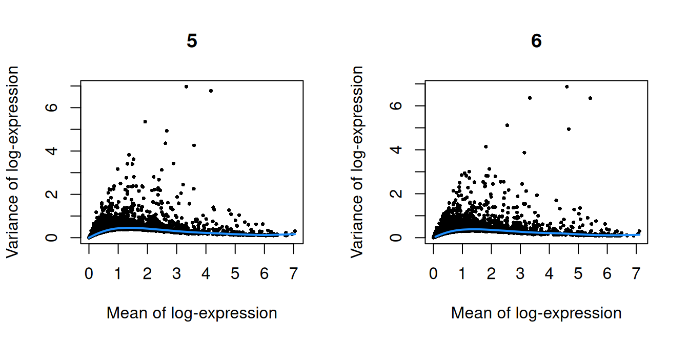
Figure 10.1: Per-gene variance as a function of the mean for the log-expression values in the Pijuan-Sala chimeric mouse embryo dataset. Each point represents a gene (black) with the mean-variance trend (blue) fitted to the variances.
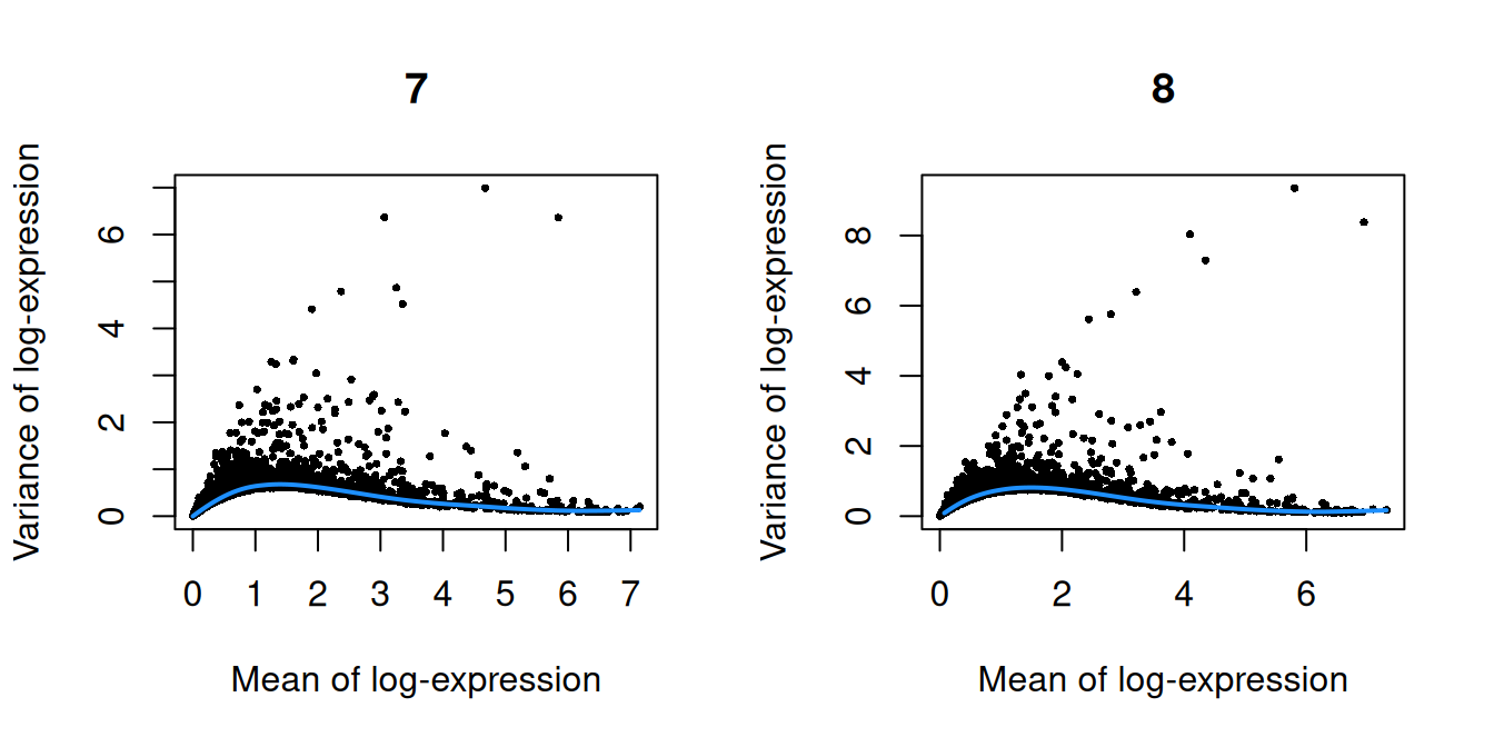
Figure 10.2: Per-gene variance as a function of the mean for the log-expression values in the Pijuan-Sala chimeric mouse embryo dataset. Each point represents a gene (black) with the mean-variance trend (blue) fitted to the variances.
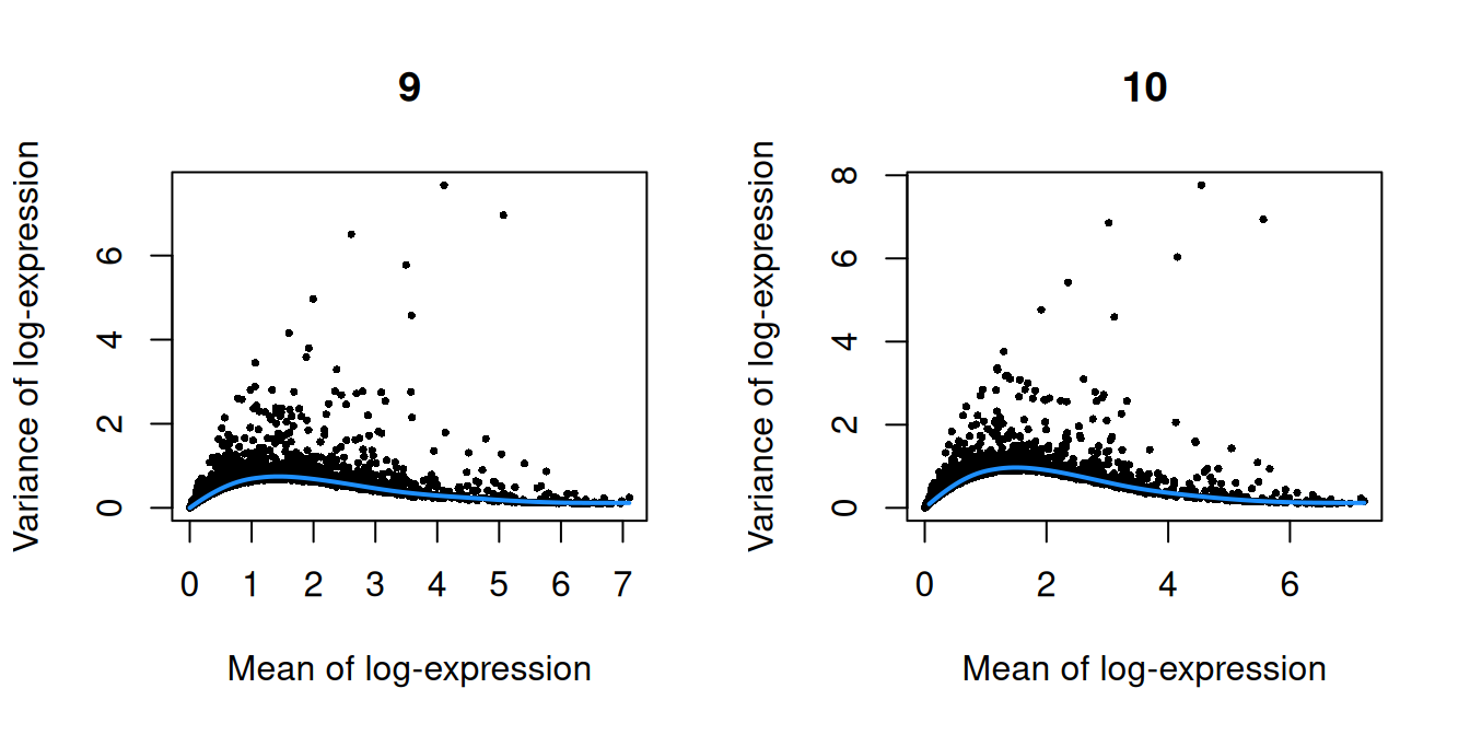
Figure 10.3: Per-gene variance as a function of the mean for the log-expression values in the Pijuan-Sala chimeric mouse embryo dataset. Each point represents a gene (black) with the mean-variance trend (blue) fitted to the variances.
10.6 Merging
We use a hierarchical merge to first merge together replicates with the same genotype, and then merge samples across different genotypes.
library(batchelor)
set.seed(01001001)
merged <- correctExperiments(sce.chimera,
    batch=sce.chimera$sample,
    subset.row=chosen.hvgs,
    PARAM=FastMnnParam(
        merge.order=list(
            list(1,3,5), # WT (3 replicates)
            list(2,4,6)  # td-Tomato (3 replicates)
        )
    )
)
We use the percentage of variance lost as a diagnostic:
##              5         6         7         8        9       10
## [1,] 0.000e+00 0.0204238 0.000e+00 0.0169321 0.000000 0.000000
## [2,] 0.000e+00 0.0007403 0.000e+00 0.0004431 0.000000 0.015455
## [3,] 3.089e-02 0.0000000 2.012e-02 0.0000000 0.000000 0.000000
## [4,] 9.042e-05 0.0000000 8.298e-05 0.0000000 0.018044 0.000000
## [5,] 4.318e-03 0.0072489 4.123e-03 0.0078254 0.003827 0.007779
10.7 Clustering
g <- buildSNNGraph(merged, use.dimred="corrected")
clusters <- igraph::cluster_louvain(g)
colLabels(merged) <- factor(clusters$membership)
We examine the distribution of cells across clusters and samples.
##        Sample
## Cluster   5   6   7   8   9  10
##      1   87  20  62  53 151  73
##      2  146  37 132 110 231 215
##      3   96  16 162 124 364 272
##      4  127  97 185 433 362 457
##      5  103  41 284 362 145 195
##      6  207  52 344 208 556 646
##      7  153  73  86  89 166 383
##      8  130  97 110  63 159 311
##      9   82  20  75  33 165 203
##      10  97  19  36  18  50  35
##      11 114  43  43  38  39 154
##      12 122  64  62  51  63 139
##      13 150  75 128  99 134 391
##      14 110  69  73  96 127 255
##      15  99  54 195 408 255 682
##      16  42  34  81  80  85 355
##      17 180  47 225 182 212 384
##      18  74  38 179 106 318 458
##      19  50  27  94  62  98 158
##      20  39  41  50  49 130 127
##      21   1   5   0  84   0  66
##      22  17   7  13  17  20  37
##      23  50  24  76  63  75 179
##      24   9   7  18  13  30  27
##      25  11  16  20   9  47  57
##      26   2   1   7   3  75 137
##      27   0   2   0  51   0   5
10.8 Dimensionality reduction
We use an external algorithm to compute nearest neighbors for greater speed.
merged <- runTSNE(merged, dimred="corrected", external_neighbors=TRUE)
merged <- runUMAP(merged, dimred="corrected", external_neighbors=TRUE)gridExtra::grid.arrange(
plotTSNE(merged, colour_by="label", text_by="label", text_colour="red"),
plotTSNE(merged, colour_by="batch")
)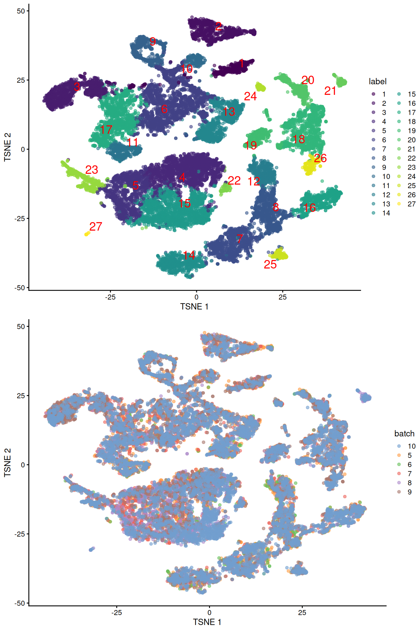
Figure 10.4: Obligatory \(t\)-SNE plots of the Pijuan-Sala chimeric mouse embryo dataset, where each point represents a cell and is colored according to the assigned cluster (top) or sample of origin (bottom).
Session Info
R version 4.6.0 RC (2026-04-17 r89917)
Platform: x86_64-pc-linux-gnu
Running under: Ubuntu 24.04.4 LTS

Matrix products: default
BLAS:   /home/biocbuild/bbs-3.23-bioc/R/lib/libRblas.so
LAPACK: /usr/lib/x86_64-linux-gnu/lapack/liblapack.so.3.12.0  LAPACK version 3.12.0

locale:
 [1] LC_CTYPE=en_US.UTF-8       LC_NUMERIC=C
 [3] LC_TIME=en_GB              LC_COLLATE=C
 [5] LC_MONETARY=en_US.UTF-8    LC_MESSAGES=en_US.UTF-8
 [7] LC_PAPER=en_US.UTF-8       LC_NAME=C
 [9] LC_ADDRESS=C               LC_TELEPHONE=C
[11] LC_MEASUREMENT=en_US.UTF-8 LC_IDENTIFICATION=C

time zone: America/New_York
tzcode source: system (glibc)

attached base packages:
[1] stats4    stats     graphics  grDevices utils     datasets  methods
[8] base

other attached packages:
 [1] batchelor_1.28.0             scran_1.40.0
 [3] scater_1.40.0                ggplot2_4.0.3
 [5] scuttle_1.22.0               MouseGastrulationData_1.25.0
 [7] SpatialExperiment_1.22.0     SingleCellExperiment_1.34.0
 [9] SummarizedExperiment_1.42.0  Biobase_2.72.0
[11] GenomicRanges_1.64.0         Seqinfo_1.2.0
[13] IRanges_2.46.0               S4Vectors_0.50.0
[15] BiocGenerics_0.58.0          generics_0.1.4
[17] MatrixGenerics_1.24.0        matrixStats_1.5.0
[19] BiocStyle_2.40.0             rebook_1.22.0

loaded via a namespace (and not attached):
  [1] RColorBrewer_1.1-3        jsonlite_2.0.0
  [3] CodeDepends_0.6.7         magrittr_2.0.5
  [5] ggbeeswarm_0.7.3          magick_2.9.1
  [7] farver_2.1.2              rmarkdown_2.31
  [9] vctrs_0.7.3               memoise_2.0.1
 [11] DelayedMatrixStats_1.34.0 htmltools_0.5.9
 [13] S4Arrays_1.12.0           AnnotationHub_4.2.0
 [15] curl_7.1.0                BiocNeighbors_2.6.0
 [17] SparseArray_1.12.0        sass_0.4.10
 [19] bslib_0.10.0              httr2_1.2.2
 [21] cachem_1.1.0              ResidualMatrix_1.22.0
 [23] igraph_2.3.0              lifecycle_1.0.5
 [25] pkgconfig_2.0.3           rsvd_1.0.5
 [27] Matrix_1.7-5              R6_2.6.1
 [29] fastmap_1.2.0             digest_0.6.39
 [31] AnnotationDbi_1.74.0      dqrng_0.4.1
 [33] irlba_2.3.7               ExperimentHub_3.2.0
 [35] RSQLite_2.4.6             beachmat_2.28.0
 [37] filelock_1.0.3            labeling_0.4.3
 [39] httr_1.4.8                abind_1.4-8
 [41] compiler_4.6.0            bit64_4.8.0
 [43] withr_3.0.2               S7_0.2.2
 [45] BiocParallel_1.46.0       viridis_0.6.5
 [47] DBI_1.3.0                 rappdirs_0.3.4
 [49] DelayedArray_0.38.0       rjson_0.2.23
 [51] bluster_1.22.0            tools_4.6.0
 [53] vipor_0.4.7               otel_0.2.0
 [55] beeswarm_0.4.0            glue_1.8.1
 [57] grid_4.6.0                Rtsne_0.17
 [59] cluster_2.1.8.2           gtable_0.3.6
 [61] BiocSingular_1.28.0       ScaledMatrix_1.20.0
 [63] metapod_1.20.0            XVector_0.52.0
 [65] ggrepel_0.9.8             BiocVersion_3.23.1
 [67] pillar_1.11.1             limma_3.68.0
 [69] BumpyMatrix_1.20.0        dplyr_1.2.1
 [71] BiocFileCache_3.2.0       lattice_0.22-9
 [73] bit_4.6.0                 tidyselect_1.2.1
 [75] locfit_1.5-9.12           Biostrings_2.80.0
 [77] knitr_1.51                gridExtra_2.3
 [79] bookdown_0.46             edgeR_4.10.0
 [81] xfun_0.57                 statmod_1.5.1
 [83] yaml_2.3.12               evaluate_1.0.5
 [85] codetools_0.2-20          tibble_3.3.1
 [87] BiocManager_1.30.27       graph_1.90.0
 [89] cli_3.6.6                 uwot_0.2.4
 [91] jquerylib_0.1.4           dichromat_2.0-0.1
 [93] Rcpp_1.1.1-1.1            dir.expiry_1.20.0
 [95] dbplyr_2.5.2              png_0.1-9
 [97] XML_3.99-0.23             parallel_4.6.0
 [99] blob_1.3.0                sparseMatrixStats_1.24.0
[101] viridisLite_0.4.3         scales_1.4.0
[103] purrr_1.2.2               crayon_1.5.3
[105] rlang_1.2.0               cowplot_1.2.0
[107] KEGGREST_1.52.0
Butler, A., P. Hoffman, P. Smibert, E. Papalexi, and R. Satija. 2018. “Integrating single-cell transcriptomic data across different conditions, technologies, and species.” Nat. Biotechnol. 36 (5): 411–20.
Büttner, Maren, Zhichao Miao, F Alexander Wolf, Sarah A Teichmann, and Fabian J Theis. 2019. “A Test Metric for Assessing Single-Cell Rna-Seq Batch Correction.” Nature Methods 16 (1): 43–49.
Chen, Y., A. T. Lun, and G. K. Smyth. 2016. “From reads to genes to pathways: differential expression analysis of RNA-Seq experiments using Rsubread and the edgeR quasi-likelihood pipeline.” F1000Res 5: 1438.
Crowell, H. L., C. Soneson, P.-L. Germain, D. Calini, L. Collin, C. Raposo, D. Malhotra, and M. D. Robinson. 2019. “On the Discovery of Population-Specific State Transitions from Multi-Sample Multi-Condition Single-Cell Rna Sequencing Data.” bioRxiv. https://doi.org/10.1101/713412.
Finak, G., J. Frelinger, W. Jiang, E. W. Newell, J. Ramey, M. M. Davis, S. A. Kalams, S. C. De Rosa, and R. Gottardo. 2014. “OpenCyto: an open source infrastructure for scalable, robust, reproducible, and automated, end-to-end flow cytometry data analysis.” PLoS Comput. Biol. 10 (8): e1003806.
Grun, D., M. J. Muraro, J. C. Boisset, K. Wiebrands, A. Lyubimova, G. Dharmadhikari, M. van den Born, et al. 2016. “De Novo Prediction of Stem Cell Identity using Single-Cell Transcriptome Data.” Cell Stem Cell 19 (2): 266–77.
Haghverdi, L., A. T. L. Lun, M. D. Morgan, and J. C. Marioni. 2018. “Batch effects in single-cell RNA-sequencing data are corrected by matching mutual nearest neighbors.” Nat. Biotechnol. 36 (5): 421–27.
Lawlor, N., J. George, M. Bolisetty, R. Kursawe, L. Sun, V. Sivakamasundari, I. Kycia, P. Robson, and M. L. Stitzel. 2017. “Single-cell transcriptomes identify human islet cell signatures and reveal cell-type-specific expression changes in type 2 diabetes.” Genome Res. 27 (2): 208–22.
Leek, J. T., W. E. Johnson, H. S. Parker, A. E. Jaffe, and J. D. Storey. 2012. “The sva package for removing batch effects and other unwanted variation in high-throughput experiments.” Bioinformatics 28 (6): 882–83.
Lin, Y., S. Ghazanfar, K. Y. X. Wang, J. A. Gagnon-Bartsch, K. K. Lo, X. Su, Z. G. Han, et al. 2019. “scMerge leverages factor analysis, stable expression, and pseudoreplication to merge multiple single-cell RNA-seq datasets.” Proc. Natl. Acad. Sci. U.S.A. 116 (20): 9775–84.
Lun, A., S. Riesenfeld, T. Andrews, T. P. Dao, T. Gomes, participants in the 1st Human Cell Atlas Jamboree, and J. Marioni. 2019. “EmptyDrops: distinguishing cells from empty droplets in droplet-based single-cell RNA sequencing data.” Genome Biol. 20 (1): 63.
Lun, A. T. L., and J. C. Marioni. 2017. “Overcoming confounding plate effects in differential expression analyses of single-cell RNA-seq data.” Biostatistics 18 (3): 451–64.
Lun, A. T. L., A. C. Richard, and J. C. Marioni. 2017. “Testing for differential abundance in mass cytometry data.” Nat. Methods 14 (7): 707–9.
McCarthy, D. J., and G. K. Smyth. 2009. “Testing significance relative to a fold-change threshold is a TREAT.” Bioinformatics 25 (6): 765–71.
Muraro, M. J., G. Dharmadhikari, D. Grun, N. Groen, T. Dielen, E. Jansen, L. van Gurp, et al. 2016. “A Single-Cell Transcriptome Atlas of the Human Pancreas.” Cell Syst 3 (4): 385–94.
Phipson, B., S. Lee, I. J. Majewski, W. S. Alexander, and G. K. Smyth. 2016. “Robust Hyperparameter Estimation Protects Against Hypervariable Genes and Improves Power to Detect Differential Expression.” Ann. Appl. Stat. 10 (2): 946–63.
Pijuan-Sala, B., J. A. Griffiths, C. Guibentif, T. W. Hiscock, W. Jawaid, F. J. Calero-Nieto, C. Mulas, et al. 2019. “A Single-Cell Molecular Map of Mouse Gastrulation and Early Organogenesis.” Nature 566 (7745): 490–95.
Richard, A. C., A. T. L. Lun, W. W. Y. Lau, B. Gottgens, J. C. Marioni, and G. M. Griffiths. 2018. “T cell cytolytic capacity is independent of initial stimulation strength.” Nat. Immunol. 19 (8): 849–58.
Ritchie, M. E., B. Phipson, D. Wu, Y. Hu, C. W. Law, W. Shi, and G. K. Smyth. 2015. “limma powers differential expression analyses for RNA-sequencing and microarray studies.” Nucleic Acids Res. 43 (7): e47.
Robinson, M. D., D. J. McCarthy, and G. K. Smyth. 2010. “edgeR: a Bioconductor package for differential expression analysis of digital gene expression data.” Bioinformatics 26 (1): 139–40.
Robinson, M. D., and A. Oshlack. 2010. “A scaling normalization method for differential expression analysis of RNA-seq data.” Genome Biol. 11 (3): R25.
Scialdone, A., Y. Tanaka, W. Jawaid, V. Moignard, N. K. Wilson, I. C. Macaulay, J. C. Marioni, and B. Gottgens. 2016. “Resolving early mesoderm diversification through single-cell expression profiling.” Nature 535 (7611): 289–93.
Segerstolpe, A., A. Palasantza, P. Eliasson, E. M. Andersson, A. C. Andreasson, X. Sun, S. Picelli, et al. 2016. “Single-Cell Transcriptome Profiling of Human Pancreatic Islets in Health and Type 2 Diabetes.” Cell Metab. 24 (4): 593–607.
Tung, P. Y., J. D. Blischak, C. J. Hsiao, D. A. Knowles, J. E. Burnett, J. K. Pritchard, and Y. Gilad. 2017. “Batch effects and the effective design of single-cell gene expression studies.” Sci. Rep. 7 (January): 39921.
Young, M. D., and S. Behjati. 2018. “SoupX Removes Ambient RNA Contamination from Droplet Based Single Cell RNA Sequencing Data.” bioRxiv.
Zheng, G. X., J. M. Terry, P. Belgrader, P. Ryvkin, Z. W. Bent, R. Wilson, S. B. Ziraldo, et al. 2017. “Massively parallel digital transcriptional profiling of single cells.” Nat Commun 8 (January): 14049.
References
Pijuan-Sala, B., J. A. Griffiths, C. Guibentif, T. W. Hiscock, W. Jawaid, F. J. Calero-Nieto, C. Mulas, et al. 2019. “A Single-Cell Molecular Map of Mouse Gastrulation and Early Organogenesis.” Nature 566 (7745): 490–95.