22 Diversity and differential abundance over time
Alpha diversity, beta diversity and differential abundance analyses from the previous chapters can be applied to longitudinal data. The difference is that samples from the same subject are paired, and the analysis has to take this into account.
In this chapter, we use an example dataset from a probiotic/placebo intervention study. The dataset includes gut microbiota samples from 22 subjects and 2 time points. The first time point was sampled before introducing a treatment.
22.1 Alpha diversity
Chapter 13 introduced alpha diversity. Here we calculate the Shannon index and visualize it by time point. Lines connect the samples of each subject.
library(miaViz)

tse <- addAlpha(tse, index = "shannon")

plotBoxplot(
    tse,
    col.var = "shannon",
    x = "time_point",
    pair.by = "subject",
    colour.by = "group",
    facet.by = "group"
)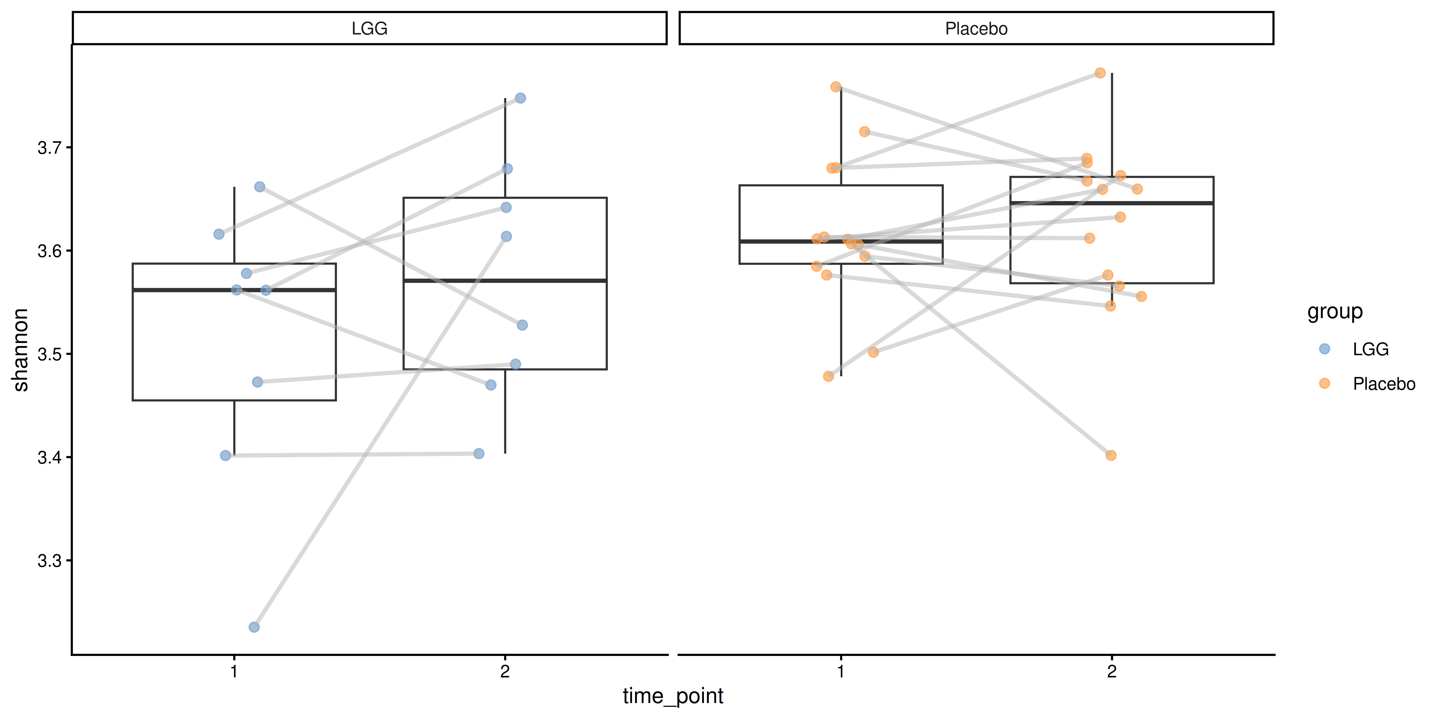
The plot does not show a clear change in either group. Because the samples are paired, we use the paired Wilcoxon test separately for each group.
df <- colData(tse) |> as.data.frame()
df <- df[order(df[["subject"]]), ]

lapply(split(df, df[["group"]]), function(x) {
    wilcox.test(
        x[x[["time_point"]] == 1, "shannon"],
        x[x[["time_point"]] == 2, "shannon"],
        paired = TRUE
    )
})
##  $LGG
##
##      Wilcoxon signed rank exact test
##
##  data:  x[x[["time_point"]] == 1, "shannon"] and x[x[["time_point"]] == 2, "shannon"]
##  V = 11, p-value = 0.4
##  alternative hypothesis: true location shift is not equal to 0
##
##
##  $Placebo
##
##      Wilcoxon signed rank exact test
##
##  data:  x[x[["time_point"]] == 1, "shannon"] and x[x[["time_point"]] == 2, "shannon"]
##  V = 49, p-value = 0.9
##  alternative hypothesis: true location shift is not equal to 0
Neither group shows a significant change in Shannon diversity between the time points. The tests above do not compare the groups. A linear mixed model can test whether the change over time differs between the groups. The time * group term includes the effects of time and group and their interaction, and (1 | subject) adds a random effect for each subject to account for the repeated measurements.
library(lmerTest)

model <- lmer(shannon ~ time * group + (1 | subject), data = df)
summary(model)
##  Linear mixed model fit by REML. t-tests use Satterthwaite's method [
##  lmerModLmerTest]
##  Formula: shannon ~ time * group + (1 | subject)
##     Data: df
##
##  REML criterion at convergence: -62.1
##
##  Scaled residuals:
##     Min     1Q Median     3Q    Max
##  -2.627 -0.486  0.038  0.494  1.486
##
##  Random effects:
##   Groups   Name        Variance Std.Dev.
##   subject  (Intercept) 0.00268  0.0518
##   Residual             0.00746  0.0864
##  Number of obs: 44, groups:  subject, 22
##
##  Fixed effects:
##                    Estimate Std. Error      df t value Pr(>|t|)
##  (Intercept)         3.4504     0.0707 27.3689   48.81   <2e-16 ***
##  time                0.0606     0.0432 20.0000    1.40    0.176
##  groupPlacebo        0.1595     0.0886 27.3689    1.80    0.083 .
##  time:groupPlacebo  -0.0551     0.0541 20.0000   -1.02    0.321
##  ---
##  Signif. codes:  0 '***' 0.001 '**' 0.01 '*' 0.05 '.' 0.1 ' ' 1
##
##  Correlation of Fixed Effects:
##              (Intr) time   grpPlc
##  time        -0.916
##  groupPlaceb -0.798  0.731
##  tim:grpPlcb  0.731 -0.798 -0.916
The interaction term “time:groupPlacebo” tests whether the change in Shannon diversity from the first to the second time point differs between the Placebo and LGG groups. The interaction is not significant, so the change in diversity does not differ between the groups.
22.2 Beta diversity
Chapter 14 introduced ordination. In longitudinal data, we can connect the samples of each subject in the ordination plot to show how the communities changed over time.
tse <- transformAssay(tse, method = "relabundance")
tse <- addMDS(tse, assay.type = "relabundance", method = "bray")

plotOrdination(
    tse,
    dimred = "MDS",
    colour.by = "group",
    pair.by = "subject",
    sort.by = "time"
)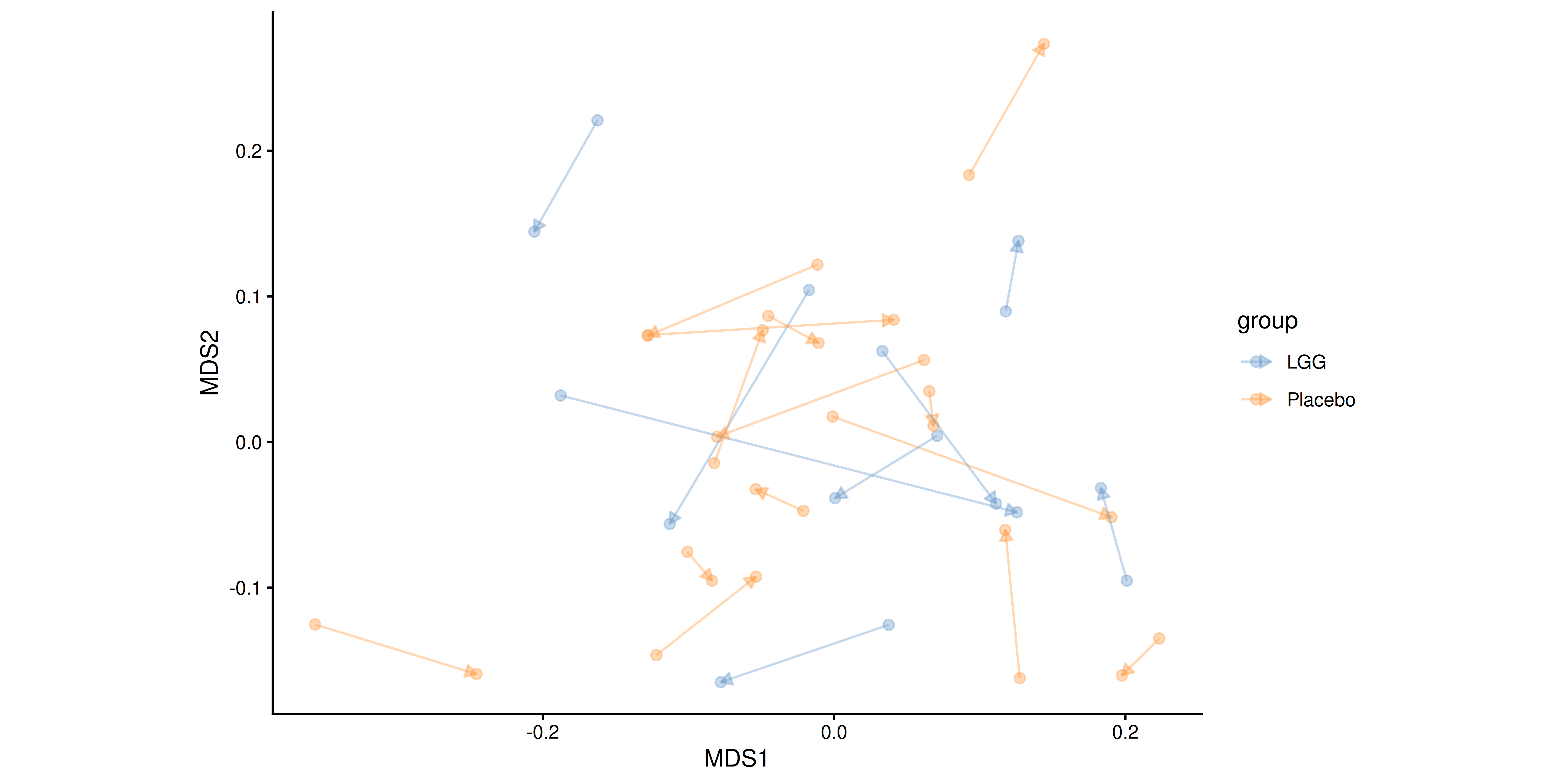
The arrows show no consistent shift that would separate the groups.
The change can also be quantified as the dissimilarity between consecutive samples of the same subject, i.e., divergence (see Section 14.2).
library(miaTime)

tse <- addStepwiseDivergence(
    tse,
    time.col = "time",
    group = "subject",
    assay.type = "relabundance",
    method = "bray"
)

plotBoxplot(
    tse,
    col.var = "divergence",
    x = "group"
)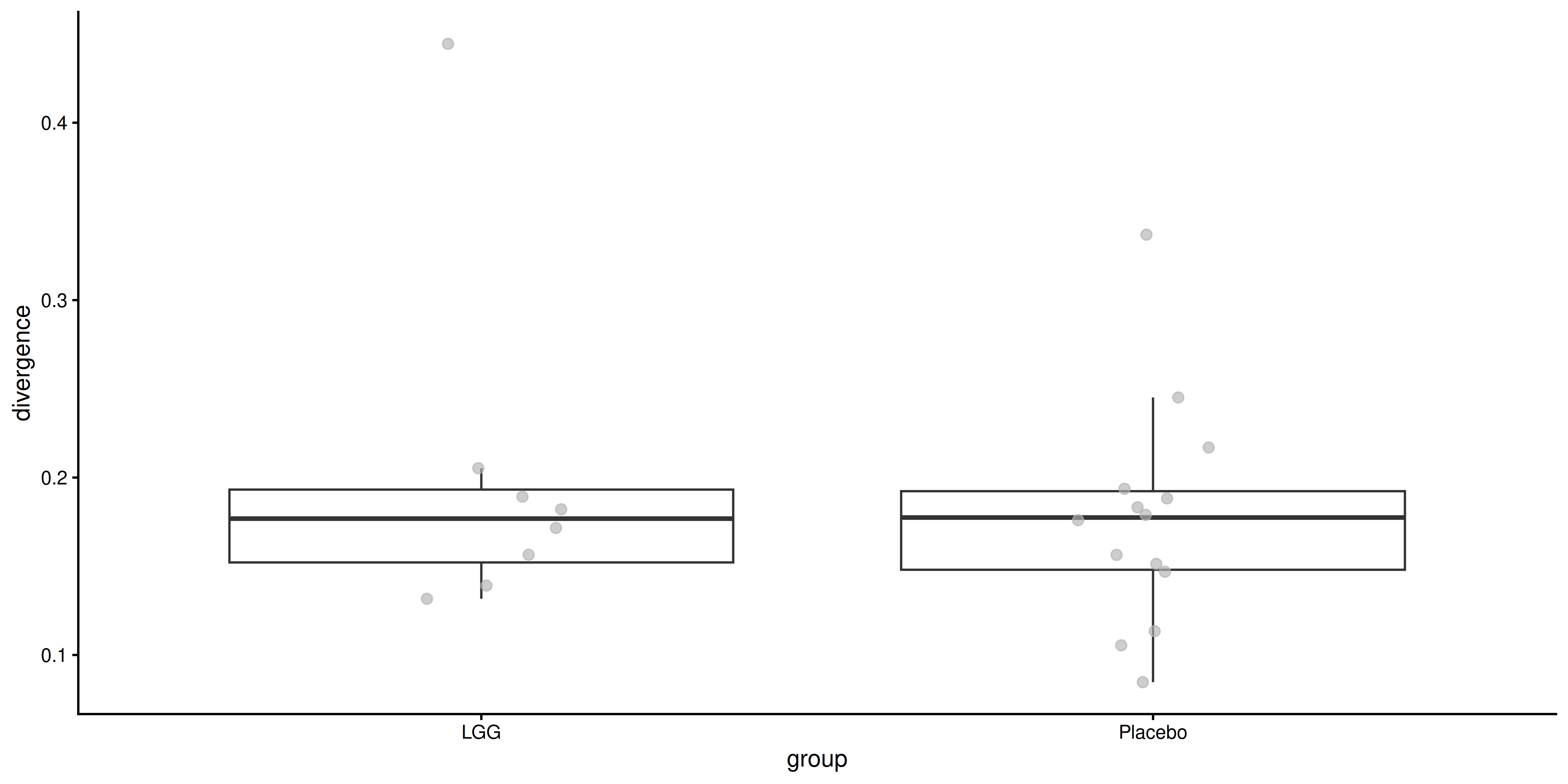
Divergence between the time points is similar in both groups.
22.3 Differential abundance
Chapter 16 introduced differential abundance analysis. With paired samples, the subject has to be included in the model. Below, we use LimROTS (Anwar et al. 2025) to test which taxa changed between the time points in the LGG group. The argument correlation_block specifies the subject, so that samples from the same subject are resampled together and their correlation is accounted for in the model. LimROTS requires log-transformed data, so we use the CLR transformation.
library(LimROTS)

tse <- transformAssay(tse, method = "rclr")
tse_lgg <- tse[, tse[["group"]] == "LGG"]

set.seed(123)
tse_lgg <- LimROTS(
    tse_lgg,
    assay.type = "rclr",
    niter = 200,
    meta.info = c("time_point", "subject"),
    group = "time_point",
    formula.str = "~ 0 + time_point",
    correlation_block = "subject",
    verbose = FALSE
)

res <- rowData(tse_lgg)[, c("corrected.logfc", "pvalue", "qvalue")]
# Sort the results
res <- res[order(res[["pvalue"]]), ]
res |> head()
##  DataFrame with 6 rows and 3 columns
##                            corrected.logfc     pvalue    qvalue
##                                  <numeric>  <numeric> <numeric>
##  Desulfovibrio et rel.           -0.381747 0.00873077  0.127019
##  Proteus et rel.                  0.355994 0.01319231  0.127019
##  Bilophila et rel.               -0.299021 0.01619231  0.127019
##  Gemella                         -0.293682 0.01653846  0.127019
##  Eggerthella lenta et rel.       -0.302522 0.01692308  0.127019
##  Aeromonas                       -0.282526 0.01748077  0.127019
corrected.logfc is the first time point minus the second, so negative values mean higher abundance at the second time point. In the LGG group, Desulfovibrio et rel. increased after the intervention. However, the result is not significant which we can see from adjusted p-values (qvalue).
LimROTS compares the levels of one categorical variable. To test whether the change differs between the groups, use a model with an interaction term as in the alpha diversity example above.