Chapter 6 Marker detection, redux
6.1 Motivation
Basic Chapter 6 described the basic process of marker detection with pairwise comparisons between clusters. Here, we describe some of the properties of each effect size, how to use custom DE methods, and a few justifications for the omission of \(p\)-values from the marker detection process.
6.2 Properties of each effect size
One of the AUC’s advantages is its robustness to the shape of the distribution of expression values within each cluster. A gene is not penalized for having a large variance so long as it does not compromise the separation between clusters. This property is demonstrated in Figure 6.1, where the AUC is not affected by the presence of an outlier subpopulation in cluster 1. By comparison, Cohen’s \(d\) decreases in the second gene, despite the fact that the outlier subpopulation does not affect the interpretation of the difference between clusters.
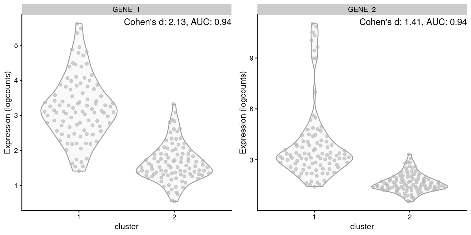
Figure 6.1: Distribution of log-expression values for two simulated genes in a pairwise comparison between clusters, in the scenario where the second gene is highly expressed in a subpopulation of cluster 1.
On the other hand, Cohen’s \(d\) accounts for the magnitude of the change in expression. All else being equal, a gene with a larger log-fold change will have a larger Cohen’s \(d\) and be prioritized during marker ranking. By comparison, the relationship between the AUC and the log-fold change is less direct. A larger log-fold change implies stronger separation and will usually lead to a larger AUC, but only up to a point - two perfectly separated distributions will have an AUC of 1 regardless of the difference in means (Figure 6.2). This reduces the resolution of the ranking and makes it more difficult to distinguish between good and very good markers.
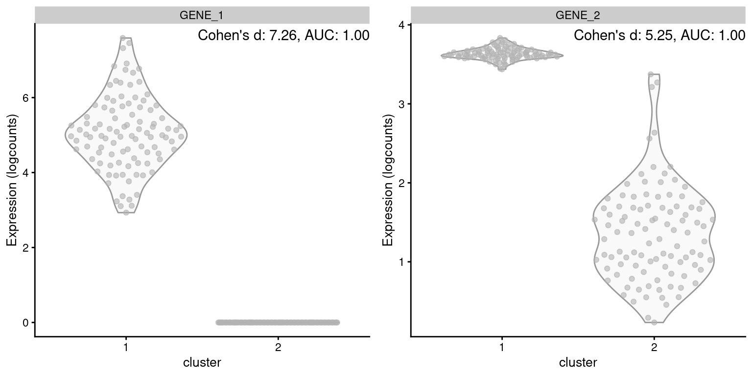
Figure 6.2: Distribution of log-expression values for two simulated genes in a pairwise comparison between clusters, in the scenario where both genes are upregulated in cluster 1 but by different magnitudes.
The log-fold change in the detected proportions is specifically designed to look for on/off changes in expression patterns.
It is relatively stringent compared to the AUC and Cohen’s \(d\), which this can lead to the loss of good candidate markers in general applications.
For example, GCG is a known marker for pancreatic alpha cells but is expressed in almost every other cell of the Lawlor et al. (2017) pancreas data (Figure 6.3) and would not be highly ranked with logFC.detected.
#--- loading ---#
library(scRNAseq)
sce.lawlor <- LawlorPancreasData()

#--- gene-annotation ---#
library(AnnotationHub)
edb <- AnnotationHub()[["AH73881"]]
anno <- select(edb, keys=rownames(sce.lawlor), keytype="GENEID",
    columns=c("SYMBOL", "SEQNAME"))
rowData(sce.lawlor) <- anno[match(rownames(sce.lawlor), anno[,1]),-1]

#--- quality-control ---#
library(scater)
stats <- perCellQCMetrics(sce.lawlor,
    subsets=list(Mito=which(rowData(sce.lawlor)$SEQNAME=="MT")))
qc <- quickPerCellQC(stats, percent_subsets="subsets_Mito_percent",
    batch=sce.lawlor$`islet unos id`)
sce.lawlor <- sce.lawlor[,!qc$discard]

#--- normalization ---#
library(scran)
set.seed(1000)
clusters <- quickCluster(sce.lawlor)
sce.lawlor <- computeSumFactors(sce.lawlor, clusters=clusters)
sce.lawlor <- logNormCounts(sce.lawlor)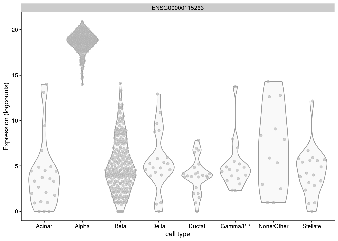
Figure 6.3: Distribution of log-normalized expression values for GCG across different pancreatic cell types in the Lawlor pancreas data.
All of these effect sizes have different interactions with log-normalization. For Cohen’s \(d\) on the log-expression values, we are directly subject to the effects described in A. Lun (2018), which can lead to spurious differences between groups. Similarly, for the AUC, we can obtain unexpected results due to the fact that normalization only equalizes the means of two distributions and not their shape. The log-fold change in the detected proportions is completely unresponsive to scaling normalization, as a zero remains so after any scaling. However, this is not necessarily problematic for marker gene detection - users can interpret this effect as retaining information about the total RNA content, analogous to spike-in normalization in Basic Section 2.4.
6.3 Using custom DE methods
We can also detect marker genes from precomputed DE statistics, allowing us to take advantage of more sophisticated tests in other Bioconductor packages such as edgeR and DESeq2.
This functionality is not commonly used - see below for an explanation - but nonetheless, we will demonstrate how one would go about applying it to the PBMC dataset.
Our strategy is to loop through each pair of clusters, performing a more-or-less standard DE analysis between pairs using the voom() approach from the limma package (Law et al. 2014).
(Specifically, we use the TREAT strategy (McCarthy and Smyth 2009) to test for log-fold changes that are significantly greater than 0.5.)
#--- loading ---#
library(DropletTestFiles)
raw.path <- getTestFile("tenx-2.1.0-pbmc4k/1.0.0/raw.tar.gz")
out.path <- file.path(tempdir(), "pbmc4k")
untar(raw.path, exdir=out.path)

library(DropletUtils)
fname <- file.path(out.path, "raw_gene_bc_matrices/GRCh38")
sce.pbmc <- read10xCounts(fname, col.names=TRUE)

#--- gene-annotation ---#
library(scater)
rownames(sce.pbmc) <- uniquifyFeatureNames(
    rowData(sce.pbmc)$ID, rowData(sce.pbmc)$Symbol)

library(EnsDb.Hsapiens.v86)
location <- mapIds(EnsDb.Hsapiens.v86, keys=rowData(sce.pbmc)$ID,
    column="SEQNAME", keytype="GENEID")

#--- cell-detection ---#
set.seed(100)
e.out <- emptyDrops(counts(sce.pbmc))
sce.pbmc <- sce.pbmc[,which(e.out$FDR <= 0.001)]

#--- quality-control ---#
stats <- perCellQCMetrics(sce.pbmc, subsets=list(Mito=which(location=="MT")))
high.mito <- isOutlier(stats$subsets_Mito_percent, type="higher")
sce.pbmc <- sce.pbmc[,!high.mito]

#--- normalization ---#
library(scran)
set.seed(1000)
clusters <- quickCluster(sce.pbmc)
sce.pbmc <- computeSumFactors(sce.pbmc, cluster=clusters)
sce.pbmc <- logNormCounts(sce.pbmc)

#--- variance-modelling ---#
set.seed(1001)
dec.pbmc <- modelGeneVarByPoisson(sce.pbmc)
top.pbmc <- getTopHVGs(dec.pbmc, prop=0.1)

#--- dimensionality-reduction ---#
set.seed(10000)
sce.pbmc <- denoisePCA(sce.pbmc, subset.row=top.pbmc, technical=dec.pbmc)

set.seed(100000)
sce.pbmc <- runTSNE(sce.pbmc, dimred="PCA")

set.seed(1000000)
sce.pbmc <- runUMAP(sce.pbmc, dimred="PCA")

#--- clustering ---#
g <- buildSNNGraph(sce.pbmc, k=10, use.dimred = 'PCA')
clust <- igraph::cluster_walktrap(g)$membership
colLabels(sce.pbmc) <- factor(clust)library(limma)
dge <- convertTo(sce.pbmc)
uclust <- unique(dge$samples$label)
all.results <- all.pairs <- list()
counter <- 1L
for (x in uclust) {
for (y in uclust) {
if (x==y) break # avoid redundant comparisons.
# Factor ordering ensures that 'x' is the not the intercept,
# so resulting fold changes can be interpreted as x/y.
subdge <- dge[,dge$samples$label %in% c(x, y)]
subdge$samples$label <- factor(subdge$samples$label, c(y, x))
design <- model.matrix(~label, subdge$samples)
# No need to normalize as we are using the size factors
# transferred from 'sce.pbmc' and converted to norm.factors.
# We also relax the filtering for the lower UMI counts.
subdge <- subdge[calculateAverage(subdge$counts) > 0.1,]
# Standard voom-limma pipeline starts here.
v <- voom(subdge, design)
fit <- lmFit(v, design)
fit <- treat(fit, lfc=0.5)
res <- topTreat(fit, n=Inf, sort.by="none")
# Filling out the genes that got filtered out with NA's.
res <- res[rownames(dge),]
rownames(res) <- rownames(dge)
all.results[[counter]] <- res
all.pairs[[counter]] <- c(x, y)
counter <- counter+1L
# Also filling the reverse comparison.
res$logFC <- -res$logFC
all.results[[counter]] <- res
all.pairs[[counter]] <- c(y, x)
counter <- counter+1L
}
}For each comparison, we store the corresponding data frame of statistics in all.results, along with the identities of the clusters involved in all.pairs.
We consolidate the pairwise DE statistics into a single marker list for each cluster with the combineMarkers() function, yielding a per-cluster DataFrame that can be interpreted in the same manner as discussed previously.
We can also specify pval.type= and direction= to control the consolidation procedure, e.g., setting pval.type="all" and direction="up" will prioritize genes that are significantly upregulated in each cluster against all other clusters.
all.pairs <- do.call(rbind, all.pairs)
combined <- combineMarkers(all.results, all.pairs, pval.field="P.Value")

# Inspecting the results for one of the clusters.
interesting.voom <- combined[["1"]]
colnames(interesting.voom)
## [1] "Top" "p.value" "FDR" "summary.logFC"
## [5] "logFC.8" "logFC.10" "logFC.2" "logFC.6"
## [9] "logFC.4" "logFC.3" "logFC.12" "logFC.11"
## [13] "logFC.7" "logFC.15" "logFC.9" "logFC.5"
## [17] "logFC.14" "logFC.13" "logFC.16"## DataFrame with 6 rows and 4 columns
## Top p.value FDR summary.logFC
## <integer> <numeric> <numeric> <numeric>
## FO538757.2 1 0 0 7.39158
## NOC2L 1 0 0 7.31139
## RPL22 1 0 0 10.50730
## RPL11 1 0 0 11.90542
## ISG15 2 0 0 7.72687
## PARK7 2 0 0 8.08160We do not routinely use custom DE methods to perform marker detection, for several reasons. Many of these methods rely on empirical Bayes shrinkage to share information across genes in the presence of limited replication. This is unnecessary when there are large numbers of “replicate” cells in each group, and does nothing to solve the fundamental \(n=1\) problem in these comparisons (Section 6.4.2). These methods also make stronger assumptions about the data (e.g., equal variances for linear models, the distribution of variances during empirical Bayes) that are more likely to be violated in noisy scRNA-seq contexts. From a practical perspective, they require more work to set up and take more time to run.
That said, some custom methods (e.g., MAST) may provide a useful point of difference from the simpler tests, in which case they can be converted into a marker detection scheme by modifing the above code. Indeed, the same code chunk can be directly applied (after switching back to the standard filtering and normalization steps inside the loop) to bulk RNA-seq experiments involving a large number of different conditions. This allows us to recycle the scran machinery to consolidate results across many pairwise comparisons for easier interpretation.
6.4 Invalidity of \(p\)-values
6.4.1 From data snooping
Given that scoreMarkers() already reports effect sizes, it is tempting to take the next step and obtain \(p\)-values for the pairwise comparisons.
Unfortunately, the \(p\)-values from the relevant tests cannot be reliably used to reject the null hypothesis.
This is because DE analysis is performed on the same data used to obtain the clusters, which represents “data dredging” (also known as fishing or data snooping).
The hypothesis of interest - are there differences between clusters? - is formulated from the data, so we are more likely to get a positive result when we re-use the data set to test that hypothesis.
The practical effect of data dredging is best illustrated with a simple simulation.
We simulate i.i.d. normal values, perform \(k\)-means clustering and test for DE between clusters of cells with pairwiseTTests().
The resulting distribution of \(p\)-values is heavily skewed towards low values (Figure 6.4).
Thus, we can detect “significant” differences between clusters even in the absence of any real substructure in the data.
This effect arises from the fact that clustering, by definition, yields groups of cells that are separated in expression space.
Testing for DE genes between clusters will inevitably yield some significant results as that is how the clusters were defined.
library(scran)
set.seed(0)
y <- matrix(rnorm(100000), ncol=200)
clusters <- kmeans(t(y), centers=2)$cluster
out <- pairwiseTTests(y, clusters)
hist(out$statistics[[1]]$p.value, col="grey80", xlab="p-value", main="")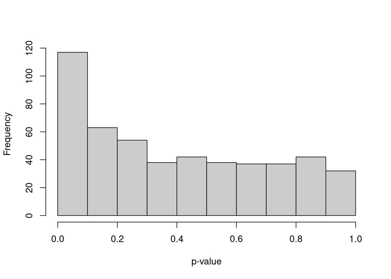
Figure 6.4: Distribution of \(p\)-values from a DE analysis between two clusters in a simulation with no true subpopulation structure.
For marker gene detection, this effect is largely harmless as the \(p\)-values are used only for ranking. However, it becomes an issue when the \(p\)-values are used to claim some statistically significant separation between clusters. Indeed, the concept of statistical significance has no obvious meaning if the clusters are empirical and cannot be stably reproduced across replicate experiments.
6.4.2 Nature of replication
The naive application of DE analysis methods will treat counts from the same cluster of cells as replicate observations. This is not the most relevant level of replication when cells are derived from the same biological sample (i.e., cell culture, animal or patient). DE analyses that treat cells as replicates fail to properly model the sample-to-sample variability (A. T. L. Lun and Marioni 2017). The latter is arguably the more important level of replication as different samples will necessarily be generated if the experiment is to be replicated. Indeed, the use of cells as replicates only masks the fact that the sample size is actually one in an experiment involving a single biological sample. This reinforces the inappropriateness of using the marker gene \(p\)-values to perform statistical inference.
Once subpopulations are identified, it is prudent to select some markers for use in validation studies with an independent replicate population of cells. A typical strategy is to identify a corresponding subset of cells that express the upregulated markers and do not express the downregulated markers. Ideally, a different technique for quantifying expression would also be used during validation, e.g., fluorescent in situ hybridisation or quantitative PCR. This confirms that the subpopulation genuinely exists and is not an artifact of the scRNA-seq protocol or the computational analysis.
6.5 Further comments
One consequence of the DE analysis strategy is that markers are defined relative to subpopulations in the same dataset. Biologically meaningful genes will not be detected if they are expressed uniformly throughout the population, e.g., T cell markers will not be detected if only T cells are present in the dataset. In practice, this is usually only a problem when the experimental data are provided without any biological context - certainly, we would hope to have some a priori idea about what cells have been captured. For most applications, it is actually desirable to avoid detecting such genes as we are interested in characterizing heterogeneity within the context of a known cell population. Continuing from the example above, the failure to detect T cell markers is of little consequence if we already know we are working with T cells. Nonetheless, if “absolute” identification of cell types is desired, some strategies for doing so are described in Basic Chapter 7.
Alternatively, marker detection can be performed by treating gene expression as a predictor variable for cluster assignment. For a pair of clusters, we can find genes that discriminate between them by performing inference with a logistic model where the outcome for each cell is whether it was assigned to the first cluster and the lone predictor is the expression of each gene. Treating the cluster assignment as the dependent variable is more philosophically pleasing in some sense, as the clusters are indeed defined from the expression data rather than being known in advance. (Note that this does not solve the data snooping problem.) In practice, this approach effectively does the same task as a Wilcoxon rank sum test in terms of quantifying separation between clusters. Logistic models have the advantage in that they can easily be extended to block on multiple nuisance variables, though this is not typically necessary in most use cases. Even more complex strategies use machine learning methods to determine which features contribute most to successful cluster classification, but this is probably unnecessary for routine analyses.
Session information
## R version 4.2.0 (2022-04-22)
## Platform: x86_64-pc-linux-gnu (64-bit)
## Running under: Ubuntu 20.04.4 LTS
##
## Matrix products: default
## BLAS:   /home/biocbuild/bbs-3.15-bioc/R/lib/libRblas.so
## LAPACK: /home/biocbuild/bbs-3.15-bioc/R/lib/libRlapack.so
##
## locale:
##  [1] LC_CTYPE=en_US.UTF-8       LC_NUMERIC=C
##  [3] LC_TIME=en_GB              LC_COLLATE=C
##  [5] LC_MONETARY=en_US.UTF-8    LC_MESSAGES=en_US.UTF-8
##  [7] LC_PAPER=en_US.UTF-8       LC_NAME=C
##  [9] LC_ADDRESS=C               LC_TELEPHONE=C
## [11] LC_MEASUREMENT=en_US.UTF-8 LC_IDENTIFICATION=C
##
## attached base packages:
## [1] stats4    stats     graphics  grDevices utils     datasets  methods
## [8] base
##
## other attached packages:
##  [1] limma_3.52.1                scran_1.24.0
##  [3] scater_1.24.0               ggplot2_3.3.6
##  [5] scuttle_1.6.2               SingleCellExperiment_1.18.0
##  [7] SummarizedExperiment_1.26.1 Biobase_2.56.0
##  [9] GenomicRanges_1.48.0        GenomeInfoDb_1.32.2
## [11] IRanges_2.30.0              S4Vectors_0.34.0
## [13] BiocGenerics_0.42.0         MatrixGenerics_1.8.0
## [15] matrixStats_0.62.0          BiocStyle_2.24.0
## [17] rebook_1.6.0
##
## loaded via a namespace (and not attached):
##  [1] bitops_1.0-7              filelock_1.0.2
##  [3] tools_4.2.0               bslib_0.3.1
##  [5] utf8_1.2.2                R6_2.5.1
##  [7] irlba_2.3.5               vipor_0.4.5
##  [9] DBI_1.1.2                 colorspace_2.0-3
## [11] withr_2.5.0               tidyselect_1.1.2
## [13] gridExtra_2.3             compiler_4.2.0
## [15] graph_1.74.0              cli_3.3.0
## [17] BiocNeighbors_1.14.0      DelayedArray_0.22.0
## [19] labeling_0.4.2            bookdown_0.26
## [21] sass_0.4.1                scales_1.2.0
## [23] rappdirs_0.3.3            stringr_1.4.0
## [25] digest_0.6.29             rmarkdown_2.14
## [27] XVector_0.36.0            pkgconfig_2.0.3
## [29] htmltools_0.5.2           sparseMatrixStats_1.8.0
## [31] highr_0.9                 fastmap_1.1.0
## [33] rlang_1.0.2               DelayedMatrixStats_1.18.0
## [35] farver_2.1.0              jquerylib_0.1.4
## [37] generics_0.1.2            jsonlite_1.8.0
## [39] BiocParallel_1.30.2       dplyr_1.0.9
## [41] RCurl_1.98-1.6            magrittr_2.0.3
## [43] BiocSingular_1.12.0       GenomeInfoDbData_1.2.8
## [45] Matrix_1.4-1              Rcpp_1.0.8.3
## [47] ggbeeswarm_0.6.0          munsell_0.5.0
## [49] fansi_1.0.3               viridis_0.6.2
## [51] lifecycle_1.0.1           edgeR_3.38.1
## [53] stringi_1.7.6             yaml_2.3.5
## [55] zlibbioc_1.42.0           grid_4.2.0
## [57] dqrng_0.3.0               parallel_4.2.0
## [59] ggrepel_0.9.1             crayon_1.5.1
## [61] dir.expiry_1.4.0          lattice_0.20-45
## [63] cowplot_1.1.1             beachmat_2.12.0
## [65] locfit_1.5-9.5            CodeDepends_0.6.5
## [67] metapod_1.4.0             knitr_1.39
## [69] pillar_1.7.0              igraph_1.3.1
## [71] codetools_0.2-18          ScaledMatrix_1.4.0
## [73] XML_3.99-0.9              glue_1.6.2
## [75] evaluate_0.15             BiocManager_1.30.18
## [77] vctrs_0.4.1               gtable_0.3.0
## [79] purrr_0.3.4               assertthat_0.2.1
## [81] xfun_0.31                 rsvd_1.0.5
## [83] viridisLite_0.4.0         tibble_3.1.7
## [85] beeswarm_0.4.0            cluster_2.1.3
## [87] statmod_1.4.36            bluster_1.6.0
## [89] ellipsis_0.3.2
References
Law, C. W., Y. Chen, W. Shi, and G. K. Smyth. 2014. “voom: Precision weights unlock linear model analysis tools for RNA-seq read counts.” Genome Biol. 15 (2): R29.
Lawlor, N., J. George, M. Bolisetty, R. Kursawe, L. Sun, V. Sivakamasundari, I. Kycia, P. Robson, and M. L. Stitzel. 2017. “Single-cell transcriptomes identify human islet cell signatures and reveal cell-type-specific expression changes in type 2 diabetes.” Genome Res. 27 (2): 208–22.
Lun, A. 2018. “Overcoming Systematic Errors Caused by Log-Transformation of Normalized Single-Cell Rna Sequencing Data.” bioRxiv.
Lun, A. T. L., and J. C. Marioni. 2017. “Overcoming confounding plate effects in differential expression analyses of single-cell RNA-seq data.” Biostatistics 18 (3): 451–64.
McCarthy, D. J., and G. K. Smyth. 2009. “Testing significance relative to a fold-change threshold is a TREAT.” Bioinformatics 25 (6): 765–71.