Chapter 13 Interactive data exploration
13.1 Motivation
Exploratory data analysis (EDA) and visualization are crucial for many aspects of data analysis such as quality control, hypothesis generation and contextual result interpretation. Single-cell ’omics datasets generated with modern high-throughput technologies are no exception, especially given their increasing size and complexity. The need for flexible and interactive platforms to explore those data from various perspectives has contributed to the increasing popularity of graphical user interfaces (GUIs) for interactive visualization.
In this chapter, we illustrate how the Bioconductor package iSEE can be used to perform some common exploratory tasks during single-cell analysis workflows.
We note that these are examples only; in practice, EDA is often context-dependent and driven by distinct motivations and hypotheses for every new data set.
To this end, iSEE provides a flexible framework that is immediately compatible with a wide range of genomics data modalities and can be easily customized to focus on key aspects of individual data sets.
13.2 Quick start
An instance of an interactive iSEE application can be launched with any data set that is stored in an object of the SummarizedExperiment class (or any class that extends it, e.g., SingleCellExperiment, DESeqDataSet, MethylSet).
In its simplest form, this is done simply by calling iSEE(sce) with the sce data object as the sole argument, as demonstrated here with the 10X PBMC dataset (Figure 13.1).
#--- loading ---#
library(DropletTestFiles)
raw.path <- getTestFile("tenx-2.1.0-pbmc4k/1.0.0/raw.tar.gz")
out.path <- file.path(tempdir(), "pbmc4k")
untar(raw.path, exdir=out.path)

library(DropletUtils)
fname <- file.path(out.path, "raw_gene_bc_matrices/GRCh38")
sce.pbmc <- read10xCounts(fname, col.names=TRUE)

#--- gene-annotation ---#
library(scater)
rownames(sce.pbmc) <- uniquifyFeatureNames(
    rowData(sce.pbmc)$ID, rowData(sce.pbmc)$Symbol)

library(EnsDb.Hsapiens.v86)
location <- mapIds(EnsDb.Hsapiens.v86, keys=rowData(sce.pbmc)$ID,
    column="SEQNAME", keytype="GENEID")

#--- cell-detection ---#
set.seed(100)
e.out <- emptyDrops(counts(sce.pbmc))
sce.pbmc <- sce.pbmc[,which(e.out$FDR <= 0.001)]

#--- quality-control ---#
stats <- perCellQCMetrics(sce.pbmc, subsets=list(Mito=which(location=="MT")))
high.mito <- isOutlier(stats$subsets_Mito_percent, type="higher")
sce.pbmc <- sce.pbmc[,!high.mito]

#--- normalization ---#
library(scran)
set.seed(1000)
clusters <- quickCluster(sce.pbmc)
sce.pbmc <- computeSumFactors(sce.pbmc, cluster=clusters)
sce.pbmc <- logNormCounts(sce.pbmc)

#--- variance-modelling ---#
set.seed(1001)
dec.pbmc <- modelGeneVarByPoisson(sce.pbmc)
top.pbmc <- getTopHVGs(dec.pbmc, prop=0.1)

#--- dimensionality-reduction ---#
set.seed(10000)
sce.pbmc <- denoisePCA(sce.pbmc, subset.row=top.pbmc, technical=dec.pbmc)

set.seed(100000)
sce.pbmc <- runTSNE(sce.pbmc, dimred="PCA")

set.seed(1000000)
sce.pbmc <- runUMAP(sce.pbmc, dimred="PCA")

#--- clustering ---#
g <- buildSNNGraph(sce.pbmc, k=10, use.dimred = 'PCA')
clust <- igraph::cluster_walktrap(g)$membership
colLabels(sce.pbmc) <- factor(clust)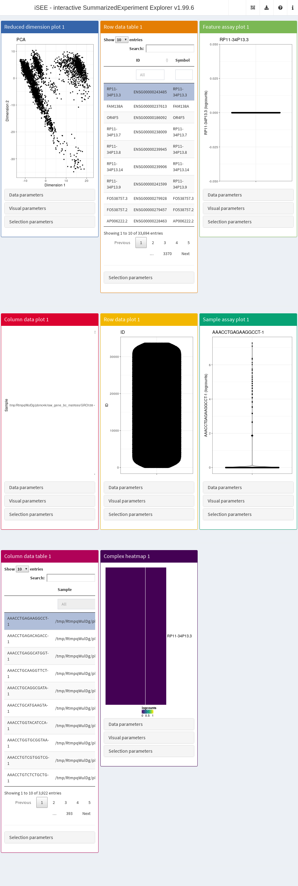
Figure 13.1: Screenshot of the iSEE application with its default initialization.
The default interface contains up to eight built-in panels, each displaying a particular aspect of the data set. The layout of panels in the interface may be altered interactively - panels can be added, removed, resized or repositioned using the “Organize panels” menu in the top right corner of the interface. The initial layout of the application can also be altered programmatically as described in the rest of this Chapter.
To familiarize themselves with the GUI, users can launch an interactive tour from the menu in the top right corner. In addition, custom tours can be written to substitute the default built-in tour. This feature is particularly useful to disseminate new data sets with accompanying bespoke explanations guiding users through the salient features of any given data set (see Section @ref{dissemination}).
It is also possible to deploy “empty” instances of iSEE apps, where any SummarizedExperiment object stored in an RDS file may be uploaded to the running application.
Once the file is uploaded, the application will import the sce object and initialize the GUI panels with the contents of the object for interactive exploration.
This type of iSEE applications is launched without specifying the sce argument, as shown in Figure 13.2.
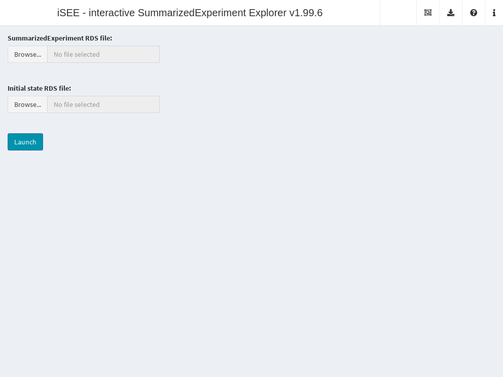
Figure 13.2: Screenshot of the iSEE application with a landing page.
13.3 Usage examples
13.3.1 Quality control
In this example, we demonstrate that an iSEE app can be configured to focus on quality control metrics.
Here, we are interested in two plots:
- The library size of each cell in decreasing order. An elbow in this plot generally reveals the transition between good quality cells and low quality cells or empty droplets.
- A dimensionality reduction result (in this case, we will pick \(t\)-SNE) where cells are colored by the log-library size. This view identifies trajectories or clusters associated with library size and can be used to diagnose QC/normalization problems. Alternatively, it could also indicate the presence of multiple cell types or states that differ in total RNA content.
In addition, by setting the ColumnSelectionSource parmaeter, any point selection made in the Column data plot panel will highlight the corresponding points in the Reduced dimension plot panel.
A user can then select the cells with either large or small library sizes to inspect their distribution in low-dimensional space.
copy.pbmc <- sce.pbmc

# Computing various QC metrics; in particular, the log10-transformed library
# size for each cell and the log-rank by decreasing library size.
library(scater)
copy.pbmc <- addPerCellQC(copy.pbmc, exprs_values="counts")
copy.pbmc$log10_total_counts <- log10(copy.pbmc$total)
copy.pbmc$total_counts_rank <- rank(-copy.pbmc$total)

initial.state <- list(
    # Configure a "Column data plot" panel
    ColumnDataPlot(YAxis="log10_total_counts",
        XAxis="Column data",
        XAxisColumnData="total_counts_rank",
        DataBoxOpen=TRUE,
        PanelId=1L),

    # Configure a "Reduced dimension plot " panel
    ReducedDimensionPlot(
        Type="TSNE",
        VisualBoxOpen=TRUE,
        DataBoxOpen=TRUE,
        ColorBy="Column data",
        ColorByColumnData="log10_total_counts",
        SelectionBoxOpen=TRUE,
        ColumnSelectionSource="ColumnDataPlot1")
)

# Prepare the app
app <- iSEE(copy.pbmc, initial=initial.state)
The configured Shiny app can then be launched with the runApp() function or by simply printing the app object (Figure 13.3).
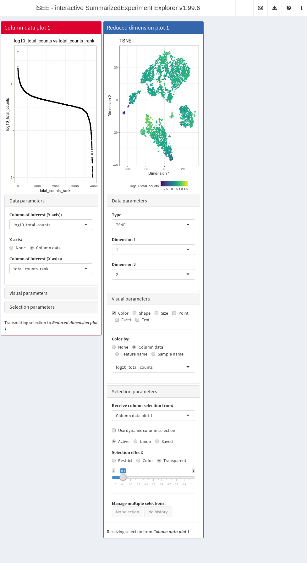
Figure 13.3: Screenshot of an iSEE application for interactive exploration of quality control metrics.
This app remains fully interactive, i.e., users can interactively control the settings and layout of the panels.
For instance, users may choose to color data points by percentage of UMI mapped to mitochondrial genes ("pct_counts_Mito") in the Reduced dimension plot.
Using the transfer of point selection between panels, users could select cells with small library sizes in the Column data plot and highlight them in the Reduced dimension plot, to investigate a possible relation between library size, clustering and proportion of reads mapped to mitochondrial genes.
13.3.2 Annotation of cell populations
In this example, we use iSEE to interactively examine the marker genes to conveniently determine cell identities.
We identify upregulated markers in each cluster (Basic Chapter 6) and collect the log-\(p\)-value for each gene in each cluster.
These are stored in the rowData slot of the SingleCellExperiment object for access by iSEE.
copy.pbmc <- sce.pbmc

library(scran)
markers.pbmc.up <- findMarkers(copy.pbmc, direction="up",
    log.p=TRUE, sorted=FALSE)

# Collate the log-p-value for each marker in a single table
all.p <- lapply(markers.pbmc.up, FUN = "[[", i="log.p.value")
all.p <- DataFrame(all.p, check.names=FALSE)
colnames(all.p) <- paste0("cluster", colnames(all.p))

# Store the table of results as row metadata
rowData(copy.pbmc) <- cbind(rowData(copy.pbmc), all.p)
The next code chunk sets up an app that contains:
- A table of feature statistics, including the log-transformed FDR of cluster markers computed above.
- A plot showing the distribution of expression values for a chosen gene in each cluster.
- A plot showing the result of the UMAP dimensionality reduction method overlaid with the expression value of a chosen gene.
Moreover, we configure the second and third panel to use the gene (i.e., row) selected in the first panel. This enables convenient examination of important markers when combined with sorting by \(p\)-value for a cluster of interest.
initial.state <- list(
    RowDataTable(PanelId=1L),

    # Configure a "Feature assay plot" panel
    FeatureAssayPlot(
        YAxisFeatureSource="RowDataTable1",
        XAxis="Column data",
        XAxisColumnData="label",
        Assay="logcounts",
        DataBoxOpen=TRUE
    ),

    # Configure a "Reduced dimension plot" panel
    ReducedDimensionPlot(
        Type="UMAP",
        ColorBy="Feature name",
        ColorByFeatureSource="RowDataTable1",
        ColorByFeatureNameAssay="logcounts"
    )
)

# Prepare the app
app <- iSEE(copy.pbmc, initial=initial.state)
After launching the application (Figure 13.4), we can then sort the table by ascending values of cluster1 to identify genes that are strong markers for cluster 1.
Then, users may select the first row in the Row statistics table and watch the second and third panel automatically update to display the most significant marker gene on the y-axis (Feature assay plot) or as a color scale overlaid on the data points (Reduced dimension plot).
Alternatively, users can simply search the table for arbitrary gene names and select known markers for visualization.
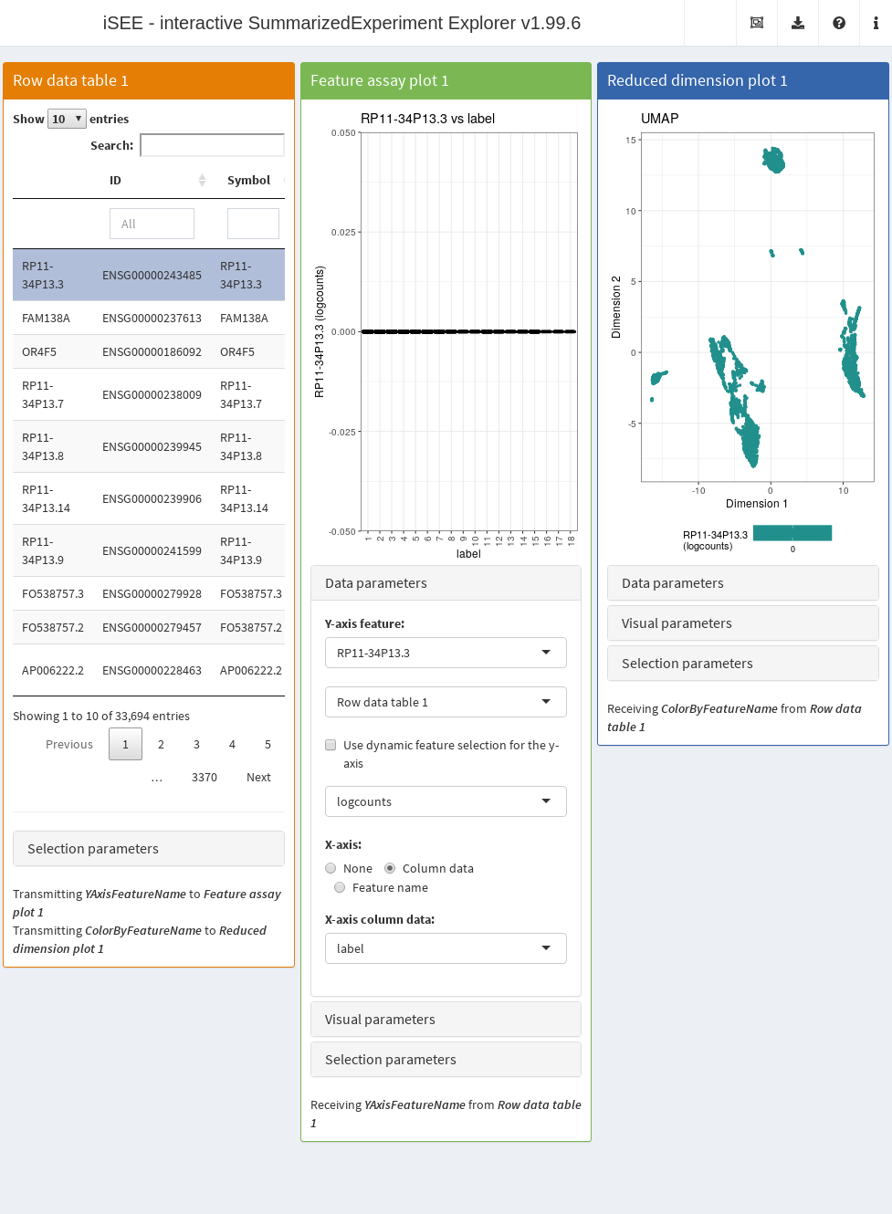
Figure 13.4: Screenshot of the iSEE application initialized for interactive exploration of population-specific marker expression.
13.3.3 Querying features of interest
So far, the plots that we have examined have represented each column (i.e., cell) as a point.
However, it is straightforward to instead represent rows as points that can be selected and transmitted to eligible panels.
This is useful for more gene-centric exploratory analyses.
To illustrate, we will add variance modelling statistics to the rowData() of our SingleCellExperiment object.
copy.pbmc <- sce.pbmc

# Adding some mean-variance information.
dec <- modelGeneVarByPoisson(copy.pbmc)
rowData(copy.pbmc) <- cbind(rowData(copy.pbmc), dec)
The next code chunk sets up an app (Figure 13.5) that contains:
- A plot showing the mean-variance trend, where each point represents a cell.
- A table of feature statistics, similar to that generated in the previous example.
- A heatmap for the genes in the first plot.
We again configure the second and third panels to respond to the selection of points in the first panel. This allows the user to select several highly variable genes at once and examine their statistics or expression profiles. More advanced users can even configure the app to start with a brush or lasso to define a selection of genes at initialization.
initial.state <- list(
    # Configure a "Feature assay plot" panel
    RowDataPlot(
        YAxis="total",
        XAxis="Row data",
        XAxisRowData="mean",
        PanelId=1L
    ),

    RowDataTable(
        RowSelectionSource="RowDataPlot1"
    ),

    # Configure a "ComplexHeatmap" panel
    ComplexHeatmapPlot(
        RowSelectionSource="RowDataPlot1",
        CustomRows=FALSE,
        ColumnData="label",
        Assay="logcounts",
        ClusterRows=TRUE,
        PanelHeight=800L,
        AssayCenterRows=TRUE
    )
)

# Prepare the app
app <- iSEE(copy.pbmc, initial=initial.state)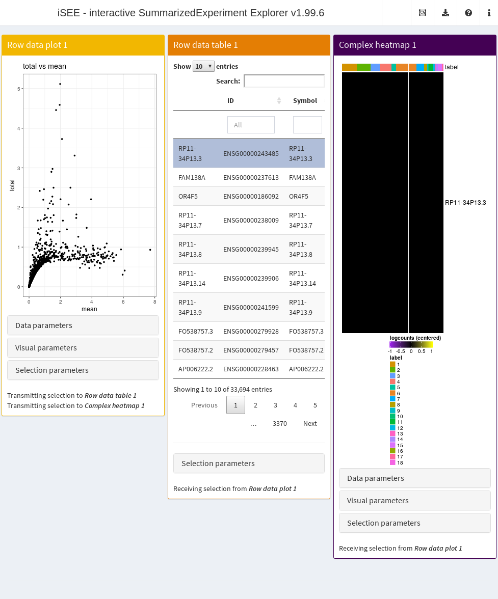
Figure 13.5: Screenshot of the iSEE application initialized for examining highly variable genes.
It is entirely possible for these row-centric panels to exist alongside the column-centric panels discussed previously. The only limitation is that row-based panels cannot transmit multi-row selections to column-based panels and vice versa. That said, a row-based panel can still transmit a single row selection to a column-based panel for, e.g., coloring by expression; this allows us to set up an app where selecting a single HVG in the mean-variance plot causes the neighboring \(t\)-SNE to be colored by the expression of the selected gene (Figure 13.6).
initial.state <- list(
    # Configure a "Feature assay plot" panel
    RowDataPlot(
        YAxis="total",
        XAxis="Row data",
        XAxisRowData="mean",
        PanelId=1L
    ),

    # Configure a "Reduced dimension plot" panel
    ReducedDimensionPlot(
        Type="TSNE",
        ColorBy="Feature name",
        ColorByFeatureSource="RowDataPlot1",
        ColorByFeatureNameAssay="logcounts"
    )
)

# Prepare the app
app <- iSEE(copy.pbmc, initial=initial.state)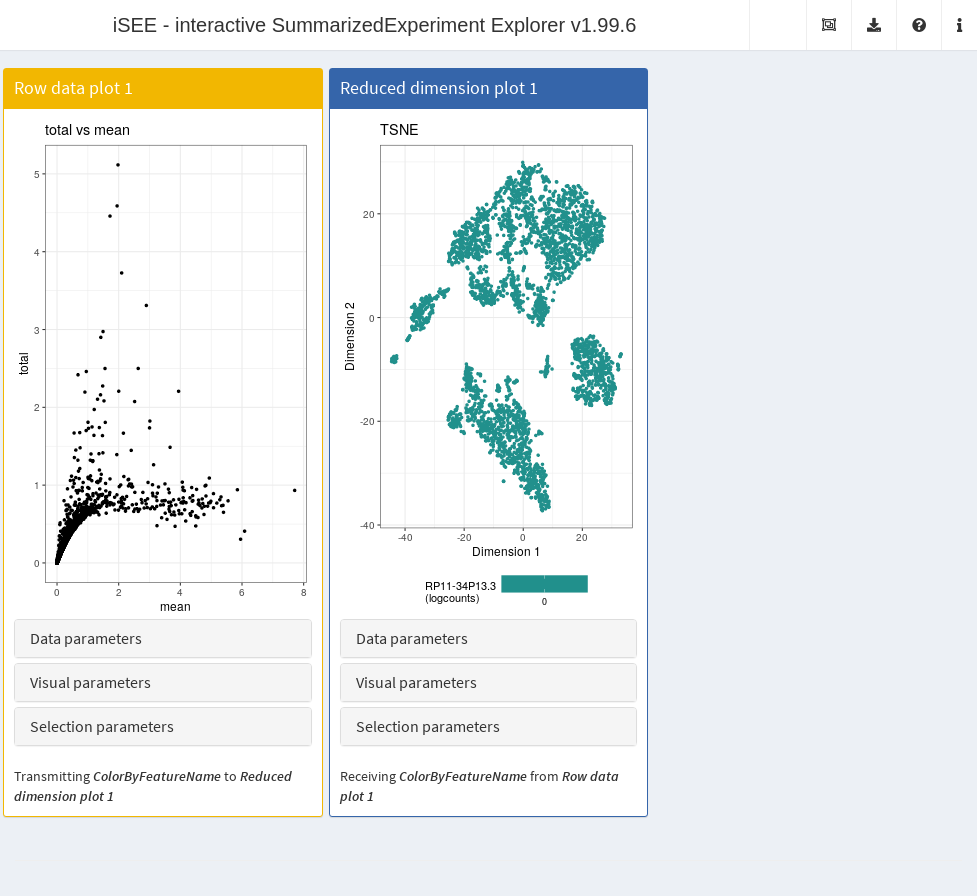
Figure 13.6: Screenshot of the iSEE application containing both row- and column-based panels.
13.4 Reproducible visualizations
The state of the iSEE application can be saved at any point to provide a snapshot of the current view of the dataset.
This is achieved by clicking on the “Display panel settings” button under the “Export” dropdown menu in the top right corner and saving an RDS file containing a serialized list of panel parameters.
Anyone with access to this file and the original SingleCellExperiment can then run iSEE to recover the same application state.
Alternatively, the code required to construct the panel parameters can be returned, which is more transparent and amenable to further modification.
This facility is most obviously useful for reproducing a perspective on the data that leads to a particular scientific conclusion;
it is also helpful for collaborations whereby different views of the same dataset can be easily transferred between analysts.
iSEE also keeps a record of the R commands used to generate each figure and table in the app.
This information is readily available via the “Extract the R code” button under the “Export” dropdown menu.
By copying the code displayed in the modal window and executing it in the R session from which the iSEE app was launched, a user can exactly reproduce all plots currently displayed in the GUI.
In this manner, a user can use iSEE to rapidly prototype plots of interest without having to write the associated boilerplate, after which they can then copy the code in an R script for fine-tuning.
Of course, the user can also save the plots and tables directly for further adjustment with other tools.
13.5 Dissemination of analysis results
iSEE provides a powerful avenue for disseminating results through a “guided tour” of the dataset.
This involves writing a step-by-step walkthrough of the different panels with explanations to facilitate their interpretation.
All that is needed to add a tour to an iSEE instance is a data frame with two columns named “element” and “intro”; the first column declares the UI element to highlight in each step of the tour, and the second one contains the text to display at that step.
This data frame must then be provided to the iSEE() function via the tour argument.
Below we demonstrate the implementation of a simple tour that takes users through the two panels that compose a GUI and trains them to use the collapsible boxes.
tour <- data.frame(
    element = c(
        "#Welcome",
        "#ReducedDimensionPlot1",
        "#ColumnDataPlot1",
        "#ColumnDataPlot1_DataBoxOpen",
        "#Conclusion"),
    intro = c(
        "Welcome to this tour!",
        "This is a <i>Reduced dimension plot.</i>",
        "And this is a <i>Column data plot.</i>",
        "<b>Action:</b> Click on this collapsible box to open and close it.",
        "Thank you for taking this tour!"),
    stringsAsFactors = FALSE)

initial.state <- list(
    ReducedDimensionPlot(PanelWidth=6L),
    ColumnDataPlot(PanelWidth=6L)
)
The preconfigured Shiny app can then be loaded with the tour and launched to obtain Figure 13.7. Note that the viewer is free to leave the interactive tour at any time and explore the data from their own perspective. Examples of advanced tours showcasing a selection of published data sets can be found at https://github.com/iSEE/iSEE2018.
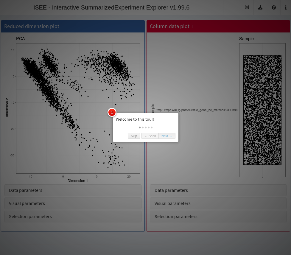
Figure 13.7: Screenshot of the iSEE application initialized with a tour.
13.6 Additional resources
For demonstration and inspiration, we refer readers to the following examples of deployed applications:
- Use cases accompanying the published article: https://marionilab.cruk.cam.ac.uk/ (source code: https://github.com/iSEE/iSEE2018)
- Examples of
iSEEin production: http://www.teichlab.org/singlecell-treg - Other examples as source code:
- Gallery of examples notebooks to reproduce analyses on public data: https://github.com/iSEE/iSEE_instances
- Gallery of example custom panels: https://github.com/iSEE/iSEE_custom
Session Info
R version 4.2.0 (2022-04-22)
Platform: x86_64-pc-linux-gnu (64-bit)
Running under: Ubuntu 20.04.4 LTS

Matrix products: default
BLAS:   /home/biocbuild/bbs-3.15-bioc/R/lib/libRblas.so
LAPACK: /home/biocbuild/bbs-3.15-bioc/R/lib/libRlapack.so

locale:
 [1] LC_CTYPE=en_US.UTF-8       LC_NUMERIC=C
 [3] LC_TIME=en_GB              LC_COLLATE=C
 [5] LC_MONETARY=en_US.UTF-8    LC_MESSAGES=en_US.UTF-8
 [7] LC_PAPER=en_US.UTF-8       LC_NAME=C
 [9] LC_ADDRESS=C               LC_TELEPHONE=C
[11] LC_MEASUREMENT=en_US.UTF-8 LC_IDENTIFICATION=C

attached base packages:
[1] stats4    stats     graphics  grDevices utils     datasets  methods
[8] base

other attached packages:
 [1] scran_1.24.0                scater_1.24.0
 [3] ggplot2_3.3.6               scuttle_1.6.2
 [5] iSEE_2.8.0                  SingleCellExperiment_1.18.0
 [7] SummarizedExperiment_1.26.1 Biobase_2.56.0
 [9] GenomicRanges_1.48.0        GenomeInfoDb_1.32.2
[11] IRanges_2.30.0              S4Vectors_0.34.0
[13] BiocGenerics_0.42.0         MatrixGenerics_1.8.0
[15] matrixStats_0.62.0          BiocStyle_2.24.0
[17] rebook_1.6.0

loaded via a namespace (and not attached):
  [1] circlize_0.4.15           igraph_1.3.1
  [3] shinydashboard_0.7.2      splines_4.2.0
  [5] BiocParallel_1.30.2       digest_0.6.29
  [7] foreach_1.5.2             htmltools_0.5.2
  [9] viridis_0.6.2             fansi_1.0.3
 [11] magrittr_2.0.3            ScaledMatrix_1.4.0
 [13] cluster_2.1.3             doParallel_1.0.17
 [15] limma_3.52.1              ComplexHeatmap_2.12.0
 [17] colorspace_2.0-3          rappdirs_0.3.3
 [19] ggrepel_0.9.1             xfun_0.31
 [21] dplyr_1.0.9               crayon_1.5.1
 [23] RCurl_1.98-1.6            jsonlite_1.8.0
 [25] graph_1.74.0              iterators_1.0.14
 [27] glue_1.6.2                gtable_0.3.0
 [29] zlibbioc_1.42.0           XVector_0.36.0
 [31] GetoptLong_1.0.5          DelayedArray_0.22.0
 [33] BiocSingular_1.12.0       shape_1.4.6
 [35] scales_1.2.0              edgeR_3.38.1
 [37] DBI_1.1.2                 miniUI_0.1.1.1
 [39] Rcpp_1.0.8.3              viridisLite_0.4.0
 [41] xtable_1.8-4              clue_0.3-60
 [43] dqrng_0.3.0               rsvd_1.0.5
 [45] DT_0.23                   metapod_1.4.0
 [47] htmlwidgets_1.5.4         dir.expiry_1.4.0
 [49] RColorBrewer_1.1-3        shinyAce_0.4.2
 [51] ellipsis_0.3.2            pkgconfig_2.0.3
 [53] XML_3.99-0.9              CodeDepends_0.6.5
 [55] sass_0.4.1                locfit_1.5-9.5
 [57] utf8_1.2.2                tidyselect_1.1.2
 [59] rlang_1.0.2               later_1.3.0
 [61] munsell_0.5.0             tools_4.2.0
 [63] cli_3.3.0                 generics_0.1.2
 [65] rintrojs_0.3.0            evaluate_0.15
 [67] stringr_1.4.0             fastmap_1.1.0
 [69] yaml_2.3.5                knitr_1.39
 [71] purrr_0.3.4               nlme_3.1-157
 [73] sparseMatrixStats_1.8.0   mime_0.12
 [75] compiler_4.2.0            beeswarm_0.4.0
 [77] filelock_1.0.2            png_0.1-7
 [79] statmod_1.4.36            tibble_3.1.7
 [81] bslib_0.3.1               stringi_1.7.6
 [83] highr_0.9                 lattice_0.20-45
 [85] bluster_1.6.0             Matrix_1.4-1
 [87] shinyjs_2.1.0             vctrs_0.4.1
 [89] pillar_1.7.0              lifecycle_1.0.1
 [91] BiocManager_1.30.18       jquerylib_0.1.4
 [93] GlobalOptions_0.1.2       BiocNeighbors_1.14.0
 [95] bitops_1.0-7              irlba_2.3.5
 [97] httpuv_1.6.5              R6_2.5.1
 [99] bookdown_0.26             promises_1.2.0.1
[101] gridExtra_2.3             vipor_0.4.5
[103] codetools_0.2-18          colourpicker_1.1.1
[105] assertthat_0.2.1          fontawesome_0.2.2
[107] rjson_0.2.21              shinyWidgets_0.7.0
[109] withr_2.5.0               GenomeInfoDbData_1.2.8
[111] mgcv_1.8-40               parallel_4.2.0
[113] grid_4.2.0                beachmat_2.12.0
[115] rmarkdown_2.14            DelayedMatrixStats_1.18.0
[117] shiny_1.7.1               ggbeeswarm_0.6.0