Chapter 8 Cross-annotating human pancreas
8.1 Loading the data
We load the Muraro et al. (2016) dataset as our reference, removing unlabelled cells or cells without a clear label.
library(scRNAseq)
sceM <- MuraroPancreasData()
sceM <- sceM[,!is.na(sceM$label) & sceM$label!="unclear"]
We compute log-expression values for use in marker detection inside SingleR().
We examine the distribution of labels in this reference.
##
##      acinar       alpha        beta       delta        duct endothelial
##         219         812         448         193         245          21
##     epsilon mesenchymal          pp
##           3          80         101
We load the Grun et al. (2016) dataset as our test, applying some basic quality control to remove low-quality cells in some of the batches (see here for details).
sceG <- GrunPancreasData()

sceG <- addPerCellQC(sceG)
qc <- quickPerCellQC(colData(sceG),
    percent_subsets="altexps_ERCC_percent",
    batch=sceG$donor,
    subset=sceG$donor %in% c("D17", "D7", "D2"))
sceG <- sceG[,!qc$discard]
Technically speaking, the test dataset does not need log-expression values but we compute them anyway for convenience.
8.2 Applying the annotation
We apply SingleR() with Wilcoxon rank sum test-based marker detection to annotate the Grun dataset with the Muraro labels.
We examine the distribution of predicted labels:
##
##      acinar       alpha        beta       delta        duct endothelial
##         289         201         178          54         295           5
##     epsilon mesenchymal          pp
##           1          23          18
We can also examine the number of discarded cells for each label:
##              Lost
## Label         FALSE TRUE
##   acinar        260   29
##   alpha         200    1
##   beta          177    1
##   delta          52    2
##   duct          291    4
##   endothelial     5    0
##   epsilon         1    0
##   mesenchymal    22    1
##   pp             18    0
8.3 Diagnostics
We visualize the assignment scores for each label in Figure 8.1.
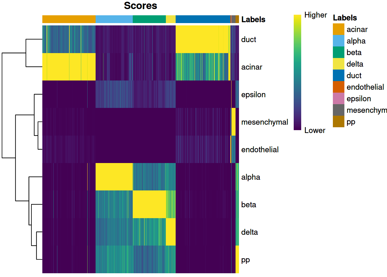
Figure 8.1: Heatmap of the (normalized) assignment scores for each cell (column) in the Grun test dataset with respect to each label (row) in the Muraro reference dataset. The final assignment for each cell is shown in the annotation bar at the top.
The delta for each cell is visualized in Figure 8.2.
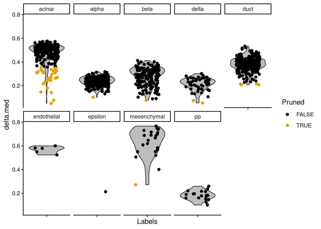
Figure 8.2: Distributions of the deltas for each cell in the Grun dataset assigned to each label in the Muraro dataset. Each cell is represented by a point; low-quality assignments that were pruned out are colored in orange.
Finally, we visualize the heatmaps of the marker genes for each label in Figure 8.3.
library(scater)
collected <- list()
all.markers <- metadata(pred.grun)$de.genes

sceG$labels <- pred.grun$labels
for (lab in unique(pred.grun$labels)) {
    collected[[lab]] <- plotHeatmap(sceG, silent=TRUE,
        order_columns_by="labels", main=lab,
        features=unique(unlist(all.markers[[lab]])))[[4]]
}
do.call(gridExtra::grid.arrange, collected)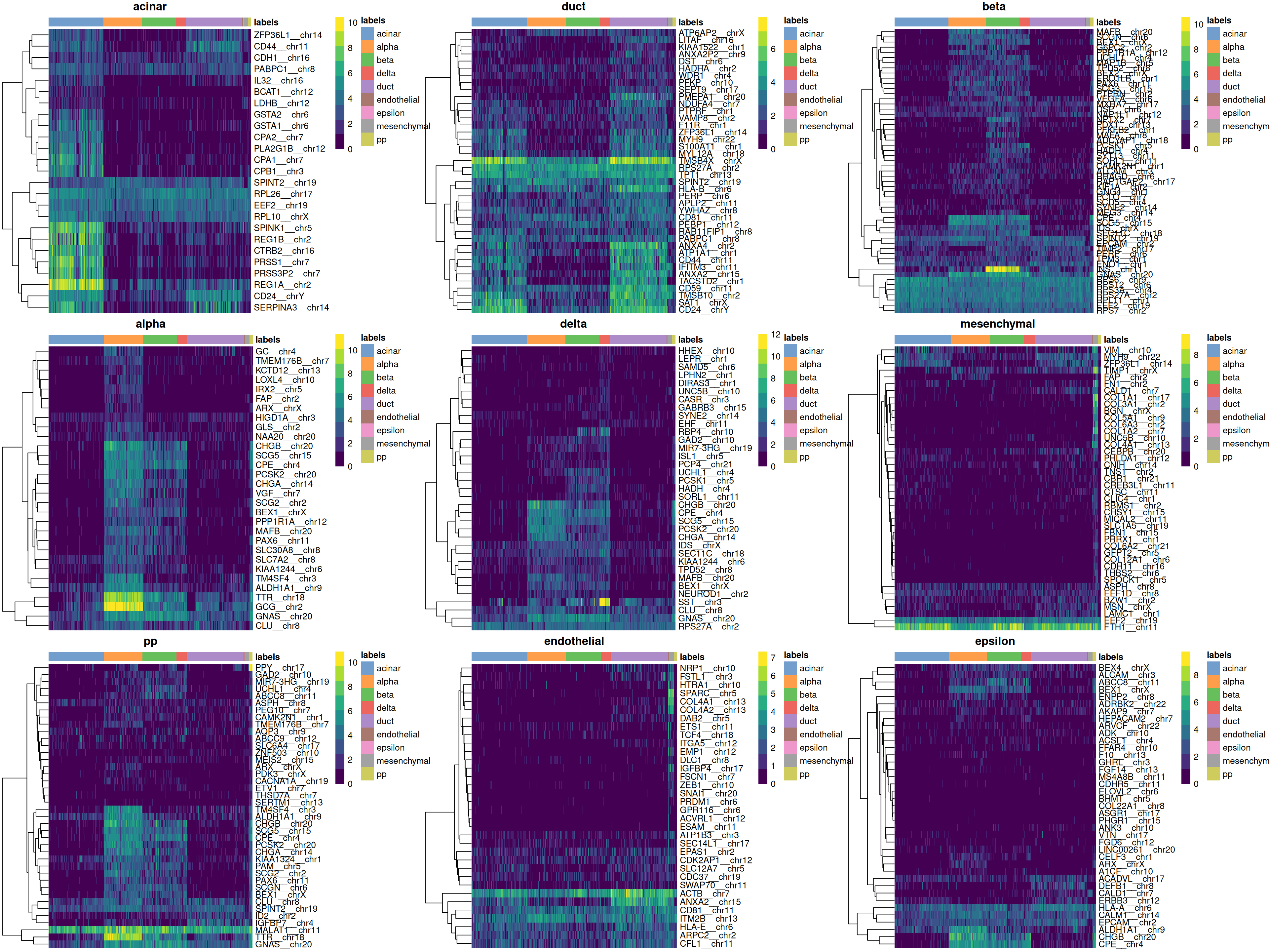
Figure 8.3: Heatmaps of log-expression values in the Grun dataset for all marker genes upregulated in each label in the Muraro reference dataset. Assigned labels for each cell are shown at the top of each plot.
8.4 Comparison to clusters
For comparison, we will perform a quick unsupervised analysis of the Grun dataset.
We model the variances using the spike-in data and we perform graph-based clustering
(increasing the resolution by dropping k=5).
library(scran)
decG <- modelGeneVarWithSpikes(sceG, "ERCC")

set.seed(1000100)
sceG <- denoisePCA(sceG, decG)

library(bluster)
sceG$cluster <- clusterRows(reducedDim(sceG), NNGraphParam(k=5))
We see that the clusters map reasonably well to the labels in Figure 8.4.
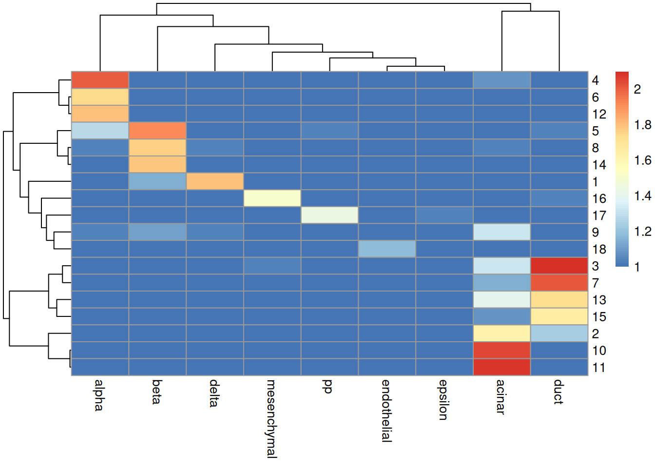
Figure 8.4: Heatmap of the log-transformed number of cells in each combination of label (column) and cluster (row) in the Grun dataset.
We proceed to the most important part of the analysis. Yes, that’s right, the \(t\)-SNE plot (Figure 8.5).
set.seed(101010100)
sceG <- runTSNE(sceG, dimred="PCA")
plotTSNE(sceG, colour_by="cluster", text_colour="red",
    text_by=I(pred.grun$labels))
Figure 8.5: \(t\)-SNE plot of the Grun dataset, where each point is a cell and is colored by the assigned cluster. Reference labels from the Muraro dataset are also placed on the median coordinate across all cells assigned with that label.
Session information
R Under development (unstable) (2025-10-20 r88955)
Platform: x86_64-pc-linux-gnu
Running under: Ubuntu 24.04.3 LTS

Matrix products: default
BLAS:   /home/biocbuild/bbs-3.23-bioc/R/lib/libRblas.so
LAPACK: /usr/lib/x86_64-linux-gnu/lapack/liblapack.so.3.12.0  LAPACK version 3.12.0

locale:
 [1] LC_CTYPE=en_US.UTF-8       LC_NUMERIC=C
 [3] LC_TIME=en_GB              LC_COLLATE=C
 [5] LC_MONETARY=en_US.UTF-8    LC_MESSAGES=en_US.UTF-8
 [7] LC_PAPER=en_US.UTF-8       LC_NAME=C
 [9] LC_ADDRESS=C               LC_TELEPHONE=C
[11] LC_MEASUREMENT=en_US.UTF-8 LC_IDENTIFICATION=C

time zone: America/New_York
tzcode source: system (glibc)

attached base packages:
[1] stats4    stats     graphics  grDevices utils     datasets  methods
[8] base

other attached packages:
 [1] bluster_1.21.0              scran_1.39.0
 [3] SingleR_2.13.0              scater_1.39.0
 [5] ggplot2_4.0.0               scuttle_1.21.0
 [7] scRNAseq_2.25.0             SingleCellExperiment_1.33.0
 [9] SummarizedExperiment_1.41.0 Biobase_2.71.0
[11] GenomicRanges_1.63.0        Seqinfo_1.1.0
[13] IRanges_2.45.0              S4Vectors_0.49.0
[15] BiocGenerics_0.57.0         generics_0.1.4
[17] MatrixGenerics_1.23.0       matrixStats_1.5.0
[19] BiocStyle_2.39.0            rebook_1.21.0

loaded via a namespace (and not attached):
  [1] RColorBrewer_1.1-3        jsonlite_2.0.0
  [3] CodeDepends_0.6.6         magrittr_2.0.4
  [5] ggbeeswarm_0.7.2          GenomicFeatures_1.63.1
  [7] gypsum_1.7.0              farver_2.1.2
  [9] rmarkdown_2.30            BiocIO_1.21.0
 [11] vctrs_0.6.5               DelayedMatrixStats_1.33.0
 [13] memoise_2.0.1             Rsamtools_2.27.0
 [15] RCurl_1.98-1.17           htmltools_0.5.8.1
 [17] S4Arrays_1.11.0           AnnotationHub_4.1.0
 [19] curl_7.0.0                BiocNeighbors_2.5.0
 [21] Rhdf5lib_1.33.0           SparseArray_1.11.1
 [23] rhdf5_2.55.4              sass_0.4.10
 [25] alabaster.base_1.11.1     bslib_0.9.0
 [27] alabaster.sce_1.11.0      httr2_1.2.1
 [29] cachem_1.1.0              GenomicAlignments_1.47.0
 [31] igraph_2.2.1              lifecycle_1.0.4
 [33] pkgconfig_2.0.3           rsvd_1.0.5
 [35] Matrix_1.7-4              R6_2.6.1
 [37] fastmap_1.2.0             digest_0.6.37
 [39] AnnotationDbi_1.73.0      dqrng_0.4.1
 [41] irlba_2.3.5.1             ExperimentHub_3.1.0
 [43] RSQLite_2.4.3             beachmat_2.27.0
 [45] labeling_0.4.3            filelock_1.0.3
 [47] httr_1.4.7                abind_1.4-8
 [49] compiler_4.6.0            bit64_4.6.0-1
 [51] withr_3.0.2               S7_0.2.0
 [53] BiocParallel_1.45.0       viridis_0.6.5
 [55] DBI_1.2.3                 HDF5Array_1.39.0
 [57] alabaster.ranges_1.11.0   alabaster.schemas_1.11.0
 [59] rappdirs_0.3.3            DelayedArray_0.37.0
 [61] rjson_0.2.23              tools_4.6.0
 [63] vipor_0.4.7               beeswarm_0.4.0
 [65] glue_1.8.0                h5mread_1.3.0
 [67] restfulr_0.0.16           rhdf5filters_1.23.0
 [69] grid_4.6.0                Rtsne_0.17
 [71] cluster_2.1.8.1           gtable_0.3.6
 [73] ensembldb_2.35.0          metapod_1.19.0
 [75] BiocSingular_1.27.0       ScaledMatrix_1.19.0
 [77] XVector_0.51.0            ggrepel_0.9.6
 [79] BiocVersion_3.23.1        pillar_1.11.1
 [81] limma_3.67.0              dplyr_1.1.4
 [83] BiocFileCache_3.1.0       lattice_0.22-7
 [85] rtracklayer_1.71.0        bit_4.6.0
 [87] tidyselect_1.2.1          locfit_1.5-9.12
 [89] Biostrings_2.79.1         knitr_1.50
 [91] gridExtra_2.3             scrapper_1.5.1
 [93] bookdown_0.45             ProtGenerics_1.43.0
 [95] edgeR_4.9.0               xfun_0.54
 [97] statmod_1.5.1             pheatmap_1.0.13
 [99] UCSC.utils_1.7.0          lazyeval_0.2.2
[101] yaml_2.3.10               evaluate_1.0.5
[103] codetools_0.2-20          cigarillo_1.1.0
[105] tibble_3.3.0              alabaster.matrix_1.11.0
[107] BiocManager_1.30.26       graph_1.89.0
[109] cli_3.6.5                 jquerylib_0.1.4
[111] dichromat_2.0-0.1         Rcpp_1.1.0
[113] GenomeInfoDb_1.47.0       dir.expiry_1.19.0
[115] dbplyr_2.5.1              png_0.1-8
[117] XML_3.99-0.19             parallel_4.6.0
[119] blob_1.2.4                AnnotationFilter_1.35.0
[121] sparseMatrixStats_1.23.0  bitops_1.0-9
[123] viridisLite_0.4.2         alabaster.se_1.11.0
[125] scales_1.4.0              crayon_1.5.3
[127] rlang_1.1.6               cowplot_1.2.0
[129] KEGGREST_1.51.0
Bibliography
Grun, D., M. J. Muraro, J. C. Boisset, K. Wiebrands, A. Lyubimova, G. Dharmadhikari, M. van den Born, et al. 2016. “De Novo Prediction of Stem Cell Identity using Single-Cell Transcriptome Data.” Cell Stem Cell 19 (2): 266–77.
Muraro, M. J., G. Dharmadhikari, D. Grun, N. Groen, T. Dielen, E. Jansen, L. van Gurp, et al. 2016. “A Single-Cell Transcriptome Atlas of the Human Pancreas.” Cell Syst 3 (4): 385–94.