Chapter 7 Advanced options
7.1 Preconstructed indices
Advanced users can split the SingleR() workflow into two separate training and classification steps.
This means that training (e.g., marker detection, assembling of nearest-neighbor indices) only needs to be performed once
for any reference.
The resulting data structure can then be re-used across multiple classifications with different test datasets,
provided the gene annotation in the test dataset is identical to or a superset of the genes in the training set.
To illustrate, we will consider the DICE reference dataset (Schmiedel et al. 2018) from the celldex package.
## class: SummarizedExperiment
## dim: 29914 1561
## metadata(0):
## assays(1): logcounts
## rownames(29914): ENSG00000121410 ENSG00000268895 ... ENSG00000159840
##   ENSG00000074755
## rowData names(0):
## colnames(1561): TPM_1 TPM_2 ... TPM_101 TPM_102
## colData names(3): label.main label.fine label.ont##
## B cells, naive Monocytes, CD14+
## 106 106
## Monocytes, CD16+ NK cells
## 105 105
## T cells, CD4+, TFH T cells, CD4+, Th1
## 104 104
## T cells, CD4+, Th17 T cells, CD4+, Th1_17
## 104 104
## T cells, CD4+, Th2 T cells, CD4+, memory TREG
## 104 104
## T cells, CD4+, naive T cells, CD4+, naive TREG
## 103 104
## T cells, CD4+, naive, stimulated T cells, CD8+, naive
## 102 104
## T cells, CD8+, naive, stimulated
## 102Let’s say we want to use the DICE reference to annotate the PBMC dataset from Chapter 1.
We use the trainSingleR() function to do all the necessary calculations that are independent of the test dataset.
This yields a list of various components that contains all identified marker genes
and precomputed rank indices to be used in the score calculation.
We can also turn on aggregation with aggr.ref=TRUE (Section 3.4)
to further reduce computational work.
Note that we need the identities of the genes in the test dataset (hence, test.genes=) to ensure that our chosen markers will actually be present in the test.
library(SingleR)
set.seed(2000)
trained <- trainSingleR(dice, labels=dice$label.fine,
    test.genes=rownames(sce), aggr.ref=TRUE)
We then use the trained object to annotate our dataset of interest through the classifySingleR() function.
As we can see, this yields exactly the same result as applying SingleR() directly.
The advantage here is that trained can be re-used for multiple classifySingleR() calls -
possibly on different datasets - without having to repeat unnecessary steps when the reference is unchanged.
##
##             B cells, naive           Monocytes, CD14+
##                        344                        516
##           Monocytes, CD16+                   NK cells
##                        185                        313
##         T cells, CD4+, TFH         T cells, CD4+, Th1
##                        456                        220
##        T cells, CD4+, Th17      T cells, CD4+, Th1_17
##                         59                         64
##         T cells, CD4+, Th2 T cells, CD4+, memory TREG
##                         45                        146
##       T cells, CD4+, naive  T cells, CD4+, naive TREG
##                        117                         25
##       T cells, CD8+, naive
##                        210
# Comparing to the direct approach.
set.seed(2000)
direct <- SingleR(sce, ref=dice, labels=dice$label.fine,
assay.type.test=1, aggr.ref=TRUE)
identical(pred$labels, direct$labels)## [1] TRUE7.2 Parallelization
Parallelization is an obvious approach to increasing annotation throughput.
This is done using the framework in the BiocParallel package,
which provides several options for parallelization depending on the available hardware.
On POSIX-compliant systems (i.e., Linux and MacOS), the simplest method is to use forking
by passing MulticoreParam() to the BPPARAM= argument:
library(BiocParallel)
pred2a <- SingleR(sce, ref=dice, assay.type.test=1, labels=dice$label.fine,
    BPPARAM=MulticoreParam(8)) # 8 CPUs.
Alternatively, one can use separate processes with SnowParam(),
which is slower but can be used on all systems - including Windows, our old nemesis.
pred2b <- SingleR(sce, ref=dice, assay.type.test=1, labels=dice$label.fine,
    BPPARAM=SnowParam(8))
identical(pred2a$labels, pred2b$labels)
## [1] TRUEWhen working on a cluster, passing BatchtoolsParam() to SingleR() allows us to
seamlessly interface with various job schedulers like SLURM, LSF and so on.
This permits heavy-duty parallelization across hundreds of CPUs for highly intensive jobs,
though often some configuration is required -
see the vignette for more details.
7.3 Approximate algorithms
It is possible to sacrifice accuracy to squeeze more speed out of SingleR.
The most obvious approach is to simply turn off the fine-tuning with fine.tune=FALSE,
which avoids the time-consuming fine-tuning iterations.
When the reference labels are well-separated, this is probably an acceptable trade-off.
pred3a <- SingleR(sce, ref=dice, assay.type.test=1,
    labels=dice$label.main, fine.tune=FALSE)
table(pred3a$labels)
##
## B cells Monocytes NK cells T cells, CD4+ T cells, CD8+
## 348 705 357 950 340Another approximation is based on the fact that the initial score calculation is done using a nearest-neighbors search.
By default, this is an exact seach but we can switch to an approximate algorithm via the BNPARAM= argument.
In the example below, we use the Annoy algorithm
via the BiocNeighbors framework, which yields mostly similar results.
(Note, though, that the Annoy method does involve a considerable amount of overhead,
so for small jobs it will actually be slower than the exact search.)
library(BiocNeighbors)
pred3b <- SingleR(sce, ref=dice, assay.type.test=1,
    labels=dice$label.main, fine.tune=FALSE, # for comparison with pred3a.
    BNPARAM=AnnoyParam())
table(pred3a$labels, pred3b$labels)
##
## B cells Monocytes NK cells T cells, CD4+ T cells, CD8+
## B cells 348 0 0 0 0
## Monocytes 0 705 0 0 0
## NK cells 0 0 357 0 0
## T cells, CD4+ 0 0 0 950 0
## T cells, CD8+ 0 0 0 0 3407.4 Cluster-level annotation
The default philosophy of SingleR is to perform annotation of each individual cell in the test dataset. An alternative strategy is to perform annotation of aggregated profiles for groups or clusters of cells. To demonstrate, we will perform a quick-and-dirty clustering of our PBMC dataset with a variety of Bioconductor packages.
library(scuttle)
sce <- logNormCounts(sce)

library(scran)
dec <- modelGeneVarByPoisson(sce)
sce <- denoisePCA(sce, dec, subset.row=getTopHVGs(dec, n=5000))

library(bluster)
colLabels(sce) <- clusterRows(reducedDim(sce), NNGraphParam())

library(scater)
set.seed(117)
sce <- runTSNE(sce, dimred="PCA")
plotTSNE(sce, colour_by="label")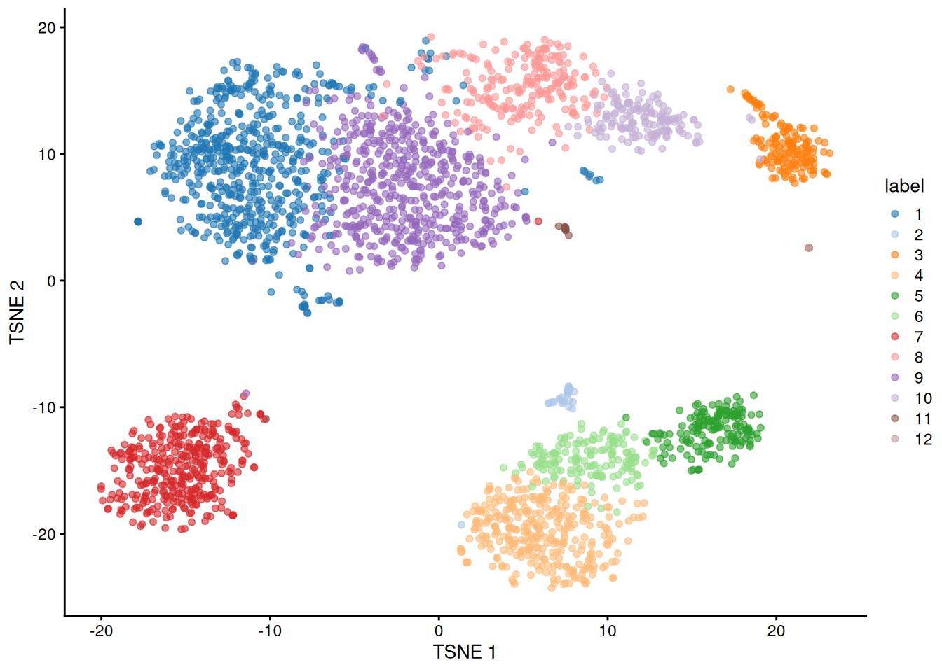
By passing clusters= to SingleR(), we direct the function to compute an aggregated profile per cluster.
Annotation is then performed on the cluster-level profiles rather than on the single-cell level.
This has the major advantage of being much faster to compute as there are obviously fewer clusters than cells;
it is also easier to interpret as it directly returns the likely cell type identity of each cluster.
## DataFrame with 12 rows and 4 columns
##                              scores        labels delta.next pruned.labels
##                            <matrix>   <character>  <numeric>   <character>
## 1   0.2064515:0.234911:0.365014:... T cells, CD4+  0.0477942 T cells, CD4+
## 2   0.2252281:0.623581:0.205190:...     Monocytes  0.3983524     Monocytes
## 3   0.0550041:0.270787:0.728557:...      NK cells  0.3343725      NK cells
## 4   0.1427138:0.781610:0.209363:...     Monocytes  0.5722475     Monocytes
## 5   0.1740008:0.756285:0.254398:...     Monocytes  0.5018874     Monocytes
## ...                             ...           ...        ...           ...
## 8   0.1527166:0.235676:0.533110:... T cells, CD4+  0.0614282 T cells, CD4+
## 9   0.2055489:0.277134:0.405779:... T cells, CD4+  0.1168394 T cells, CD4+
## 10  0.1403238:0.258656:0.605894:...      NK cells  0.0820843      NK cells
## 11  0.2535745:0.258933:0.328738:... T cells, CD4+  0.0569244 T cells, CD4+
## 12  0.0713926:0.223101:0.117047:...     Monocytes  0.1060540            NA
This approach assumes that each cluster in the test dataset corresponds to exactly one reference label.
If a cluster actually contains a mixture of multiple labels, this will not be reflected in its lone assigned label.
(We note that it would be very difficult to determine the composition of the mixture from the SingleR() scores.)
Indeed, there is no guarantee that the clustering is driven by the same factors that distinguish the reference labels,
decreasing the reliability of the annotations when novel heterogeneity is present in the test dataset.
The default per-cell strategy is safer and provides more information about the ambiguity of the annotations,
which is important for closely related labels where a close correspondence between clusters and labels cannot be expected.
Session information
R version 4.6.0 RC (2026-04-17 r89917)
Platform: x86_64-pc-linux-gnu
Running under: Ubuntu 24.04.4 LTS

Matrix products: default
BLAS:   /home/biocbuild/bbs-3.24-bioc/R/lib/libRblas.so
LAPACK: /usr/lib/x86_64-linux-gnu/lapack/liblapack.so.3.12.0  LAPACK version 3.12.0

locale:
 [1] LC_CTYPE=en_US.UTF-8       LC_NUMERIC=C
 [3] LC_TIME=en_GB              LC_COLLATE=C
 [5] LC_MONETARY=en_US.UTF-8    LC_MESSAGES=en_US.UTF-8
 [7] LC_PAPER=en_US.UTF-8       LC_NAME=C
 [9] LC_ADDRESS=C               LC_TELEPHONE=C
[11] LC_MEASUREMENT=en_US.UTF-8 LC_IDENTIFICATION=C

time zone: America/New_York
tzcode source: system (glibc)

attached base packages:
[1] stats4    stats     graphics  grDevices utils     datasets  methods
[8] base

other attached packages:
 [1] scater_1.41.1               ggplot2_4.0.3
 [3] bluster_1.23.0              scran_1.41.0
 [5] scuttle_1.23.0              BiocNeighbors_2.7.0
 [7] BiocParallel_1.47.0         SingleR_2.15.0
 [9] TENxPBMCData_1.31.0         HDF5Array_1.41.0
[11] h5mread_1.5.0               rhdf5_2.57.0
[13] DelayedArray_0.39.1         SparseArray_1.13.2
[15] S4Arrays_1.13.0             abind_1.4-8
[17] Matrix_1.7-5                SingleCellExperiment_1.35.0
[19] ensembldb_2.37.0            AnnotationFilter_1.37.0
[21] GenomicFeatures_1.65.0      AnnotationDbi_1.75.0
[23] celldex_1.23.0              SummarizedExperiment_1.43.0
[25] Biobase_2.73.1              GenomicRanges_1.65.0
[27] Seqinfo_1.3.0               IRanges_2.47.0
[29] S4Vectors_0.51.1            BiocGenerics_0.59.0
[31] generics_0.1.4              MatrixGenerics_1.25.0
[33] matrixStats_1.5.0           BiocStyle_2.41.0
[35] rebook_1.23.0

loaded via a namespace (and not attached):
  [1] RColorBrewer_1.1-3        jsonlite_2.0.0
  [3] CodeDepends_0.6.7         magrittr_2.0.5
  [5] ggbeeswarm_0.7.3          gypsum_1.9.0
  [7] farver_2.1.2              rmarkdown_2.31
  [9] BiocIO_1.23.3             vctrs_0.7.3
 [11] memoise_2.0.1             Rsamtools_2.29.0
 [13] DelayedMatrixStats_1.35.0 RCurl_1.98-1.18
 [15] htmltools_0.5.9           BiocBaseUtils_1.15.0
 [17] AnnotationHub_4.3.0       curl_7.1.0
 [19] Rhdf5lib_2.1.0            sass_0.4.10
 [21] alabaster.base_1.13.0     bslib_0.10.0
 [23] httr2_1.2.2               cachem_1.1.0
 [25] GenomicAlignments_1.49.0  igraph_2.3.1
 [27] lifecycle_1.0.5           pkgconfig_2.0.3
 [29] rsvd_1.0.5                R6_2.6.1
 [31] fastmap_1.2.0             digest_0.6.39
 [33] dqrng_0.4.1               irlba_2.3.7
 [35] ExperimentHub_3.3.0       RSQLite_2.4.6
 [37] beachmat_2.29.0           labeling_0.4.3
 [39] filelock_1.0.3            httr_1.4.8
 [41] compiler_4.6.0            bit64_4.8.0
 [43] withr_3.0.2               S7_0.2.2
 [45] viridis_0.6.5             DBI_1.3.0
 [47] alabaster.ranges_1.13.0   alabaster.schemas_1.13.0
 [49] rappdirs_0.3.4            rjson_0.2.23
 [51] tools_4.6.0               vipor_0.4.7
 [53] otel_0.2.0                beeswarm_0.4.0
 [55] glue_1.8.1                restfulr_0.0.16
 [57] rhdf5filters_1.25.0       grid_4.6.0
 [59] Rtsne_0.17                cluster_2.1.8.2
 [61] gtable_0.3.6              metapod_1.21.0
 [63] BiocSingular_1.29.0       ScaledMatrix_1.21.0
 [65] XVector_0.53.0            ggrepel_0.9.8
 [67] BiocVersion_3.24.0        pillar_1.11.1
 [69] limma_3.69.0              dplyr_1.2.1
 [71] BiocFileCache_3.3.0       lattice_0.22-9
 [73] rtracklayer_1.73.0        bit_4.6.0
 [75] tidyselect_1.2.1          locfit_1.5-9.12
 [77] Biostrings_2.81.1         knitr_1.51
 [79] gridExtra_2.3             scrapper_1.7.0
 [81] bookdown_0.46             ProtGenerics_1.45.0
 [83] edgeR_4.11.0              xfun_0.57
 [85] statmod_1.5.1             UCSC.utils_1.9.0
 [87] lazyeval_0.2.3            yaml_2.3.12
 [89] evaluate_1.0.5            codetools_0.2-20
 [91] cigarillo_1.3.0           tibble_3.3.1
 [93] alabaster.matrix_1.13.0   BiocManager_1.30.27
 [95] graph_1.91.0              cli_3.6.6
 [97] jquerylib_0.1.4           dichromat_2.0-0.1
 [99] Rcpp_1.1.1-1.1            GenomeInfoDb_1.49.0
[101] dir.expiry_1.21.0         dbplyr_2.5.2
[103] png_0.1-9                 XML_3.99-0.23
[105] parallel_4.6.0            blob_1.3.0
[107] sparseMatrixStats_1.25.0  bitops_1.0-9
[109] viridisLite_0.4.3         alabaster.se_1.13.0
[111] scales_1.4.0              purrr_1.2.2
[113] crayon_1.5.3              rlang_1.2.0
[115] cowplot_1.2.0             KEGGREST_1.53.0
Bibliography
Schmiedel, Benjamin J., Divya Singh, Ariel Madrigal, Alan G. Valdovino-Gonzalez, Brandie M. White, Jose Zapardiel-Gonzalo, Brendan Ha, et al. 2018. “Impact of Genetic Polymorphisms on Human Immune Cell Gene Expression.” Cell 175 (6): 1701–1715.e16. https://doi.org/10.1016/j.cell.2018.10.022.