Chapter 10 Nestorowa mouse HSC (Smart-seq2)
10.1 Introduction
This performs an analysis of the mouse haematopoietic stem cell (HSC) dataset generated with Smart-seq2 (Nestorowa et al. 2016).
10.2 Data loading
library(AnnotationHub)
ens.mm.v97 <- AnnotationHub()[["AH73905"]]
anno <- select(ens.mm.v97, keys=rownames(sce.nest),
    keytype="GENEID", columns=c("SYMBOL", "SEQNAME"))
rowData(sce.nest) <- anno[match(rownames(sce.nest), anno$GENEID),]
After loading and annotation, we inspect the resulting SingleCellExperiment object:
## class: SingleCellExperiment
## dim: 46078 1920
## metadata(0):
## assays(1): counts
## rownames(46078): ENSMUSG00000000001 ENSMUSG00000000003 ...
##   ENSMUSG00000107391 ENSMUSG00000107392
## rowData names(3): GENEID SYMBOL SEQNAME
## colnames(1920): HSPC_007 HSPC_013 ... Prog_852 Prog_810
## colData names(9): gate broad ... projected metrics
## reducedDimNames(1): diffusion
## mainExpName: endogenous
## altExpNames(2): ERCC FACS
10.3 Quality control
For some reason, no mitochondrial transcripts are available, so we will perform quality control using the spike-in proportions only.
library(scater)
stats <- perCellQCMetrics(sce.nest)
qc <- quickPerCellQC(stats, percent_subsets="altexps_ERCC_percent")
sce.nest <- sce.nest[,!qc$discard]
We examine the number of cells discarded for each reason.
##              low_lib_size            low_n_features high_altexps_ERCC_percent
##                       146                        28                       241
##                   discard
##                       264
We create some diagnostic plots for each metric (Figure 10.1).
colData(unfiltered) <- cbind(colData(unfiltered), stats)
unfiltered$discard <- qc$discard

gridExtra::grid.arrange(
    plotColData(unfiltered, y="sum", colour_by="discard") +
        scale_y_log10() + ggtitle("Total count"),
    plotColData(unfiltered, y="detected", colour_by="discard") +
        scale_y_log10() + ggtitle("Detected features"),
    plotColData(unfiltered, y="altexps_ERCC_percent",
        colour_by="discard") + ggtitle("ERCC percent"),
    ncol=2
)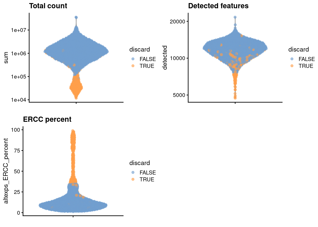
Figure 10.1: Distribution of each QC metric across cells in the Nestorowa HSC dataset. Each point represents a cell and is colored according to whether that cell was discarded.
10.4 Normalization
library(scran)
set.seed(101000110)
clusters <- quickCluster(sce.nest)
sce.nest <- computeSumFactors(sce.nest, clusters=clusters)
sce.nest <- logNormCounts(sce.nest)
We examine some key metrics for the distribution of size factors, and compare it to the library sizes as a sanity check (Figure 10.2).
##    Min. 1st Qu.  Median    Mean 3rd Qu.    Max.
## 0.039 0.420 0.743 1.000 1.249 16.789plot(librarySizeFactors(sce.nest), sizeFactors(sce.nest), pch=16,
xlab="Library size factors", ylab="Deconvolution factors", log="xy")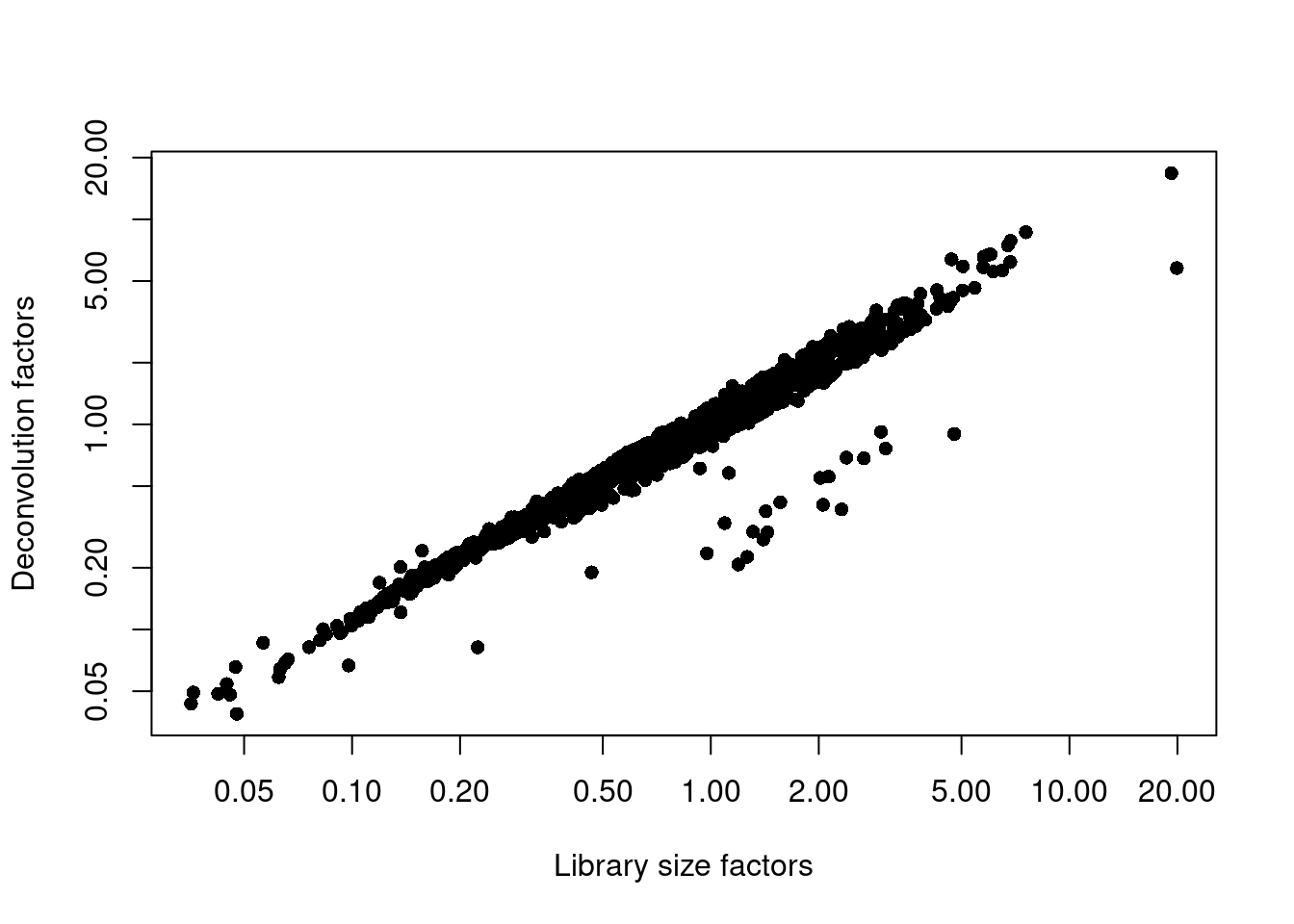
Figure 10.2: Relationship between the library size factors and the deconvolution size factors in the Nestorowa HSC dataset.
10.5 Variance modelling
We use the spike-in transcripts to model the technical noise as a function of the mean (Figure 10.3).
set.seed(00010101)
dec.nest <- modelGeneVarWithSpikes(sce.nest, "ERCC")
top.nest <- getTopHVGs(dec.nest, prop=0.1)plot(dec.nest$mean, dec.nest$total, pch=16, cex=0.5,
xlab="Mean of log-expression", ylab="Variance of log-expression")
curfit <- metadata(dec.nest)
curve(curfit$trend(x), col='dodgerblue', add=TRUE, lwd=2)
points(curfit$mean, curfit$var, col="red")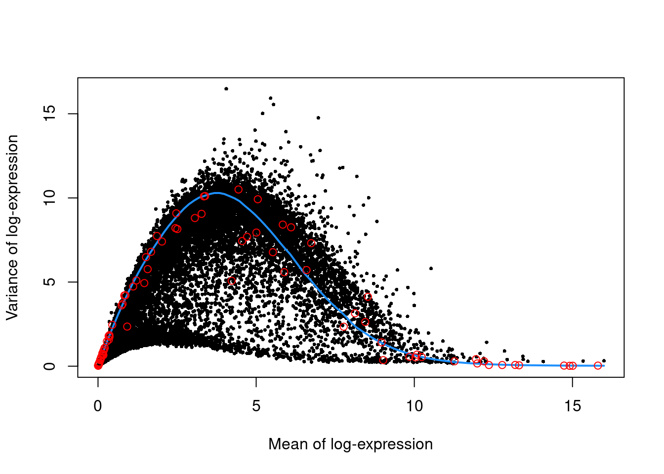
Figure 10.3: Per-gene variance as a function of the mean for the log-expression values in the Nestorowa HSC dataset. Each point represents a gene (black) with the mean-variance trend (blue) fitted to the spike-ins (red).
10.6 Dimensionality reduction
set.seed(101010011)
sce.nest <- denoisePCA(sce.nest, technical=dec.nest, subset.row=top.nest)
sce.nest <- runTSNE(sce.nest, dimred="PCA")
We check that the number of retained PCs is sensible.
## [1] 910.7 Clustering
snn.gr <- buildSNNGraph(sce.nest, use.dimred="PCA")
colLabels(sce.nest) <- factor(igraph::cluster_walktrap(snn.gr)$membership)##
## 1 2 3 4 5 6 7 8 9 10
## 198 319 208 147 221 182 21 209 74 77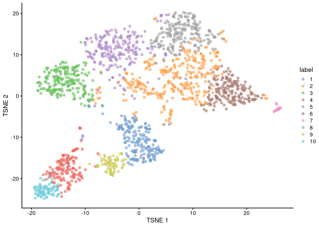
Figure 10.4: Obligatory \(t\)-SNE plot of the Nestorowa HSC dataset, where each point represents a cell and is colored according to the assigned cluster.
10.8 Marker gene detection
markers <- findMarkers(sce.nest, colLabels(sce.nest),
    test.type="wilcox", direction="up", lfc=0.5,
    row.data=rowData(sce.nest)[,"SYMBOL",drop=FALSE])
To illustrate the manual annotation process, we examine the marker genes for one of the clusters. Upregulation of Car2, Hebp1 amd hemoglobins indicates that cluster 10 contains erythroid precursors.
chosen <- markers[['10']]
best <- chosen[chosen$Top <= 10,]
aucs <- getMarkerEffects(best, prefix="AUC")
rownames(aucs) <- best$SYMBOL

library(pheatmap)
pheatmap(aucs, color=viridis::plasma(100))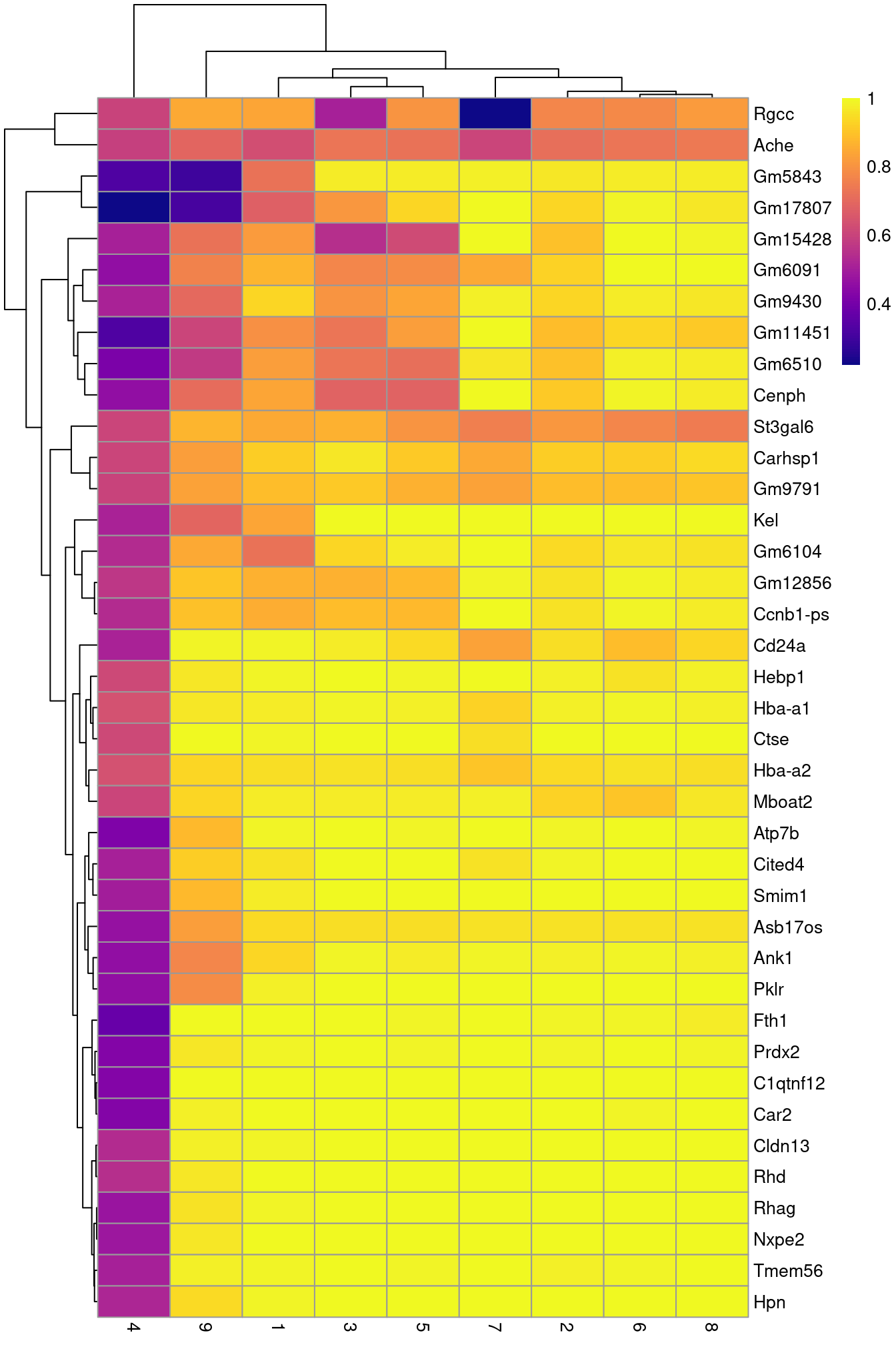
Figure 10.5: Heatmap of the AUCs for the top marker genes in cluster 10 compared to all other clusters.
10.9 Cell type annotation
library(SingleR)
mm.ref <- MouseRNAseqData()

# Renaming to symbols to match with reference row names.
renamed <- sce.nest
rownames(renamed) <- uniquifyFeatureNames(rownames(renamed),
    rowData(sce.nest)$SYMBOL)
labels <- SingleR(renamed, mm.ref, labels=mm.ref$label.fine)
Most clusters are not assigned to any single lineage (Figure 10.6), which is perhaps unsurprising given that HSCs are quite different from their terminal fates. Cluster 10 is considered to contain erythrocytes, which is roughly consistent with our conclusions from the marker gene analysis above.
tab <- table(labels$labels, colLabels(sce.nest))
pheatmap(log10(tab+10), color=viridis::viridis(100))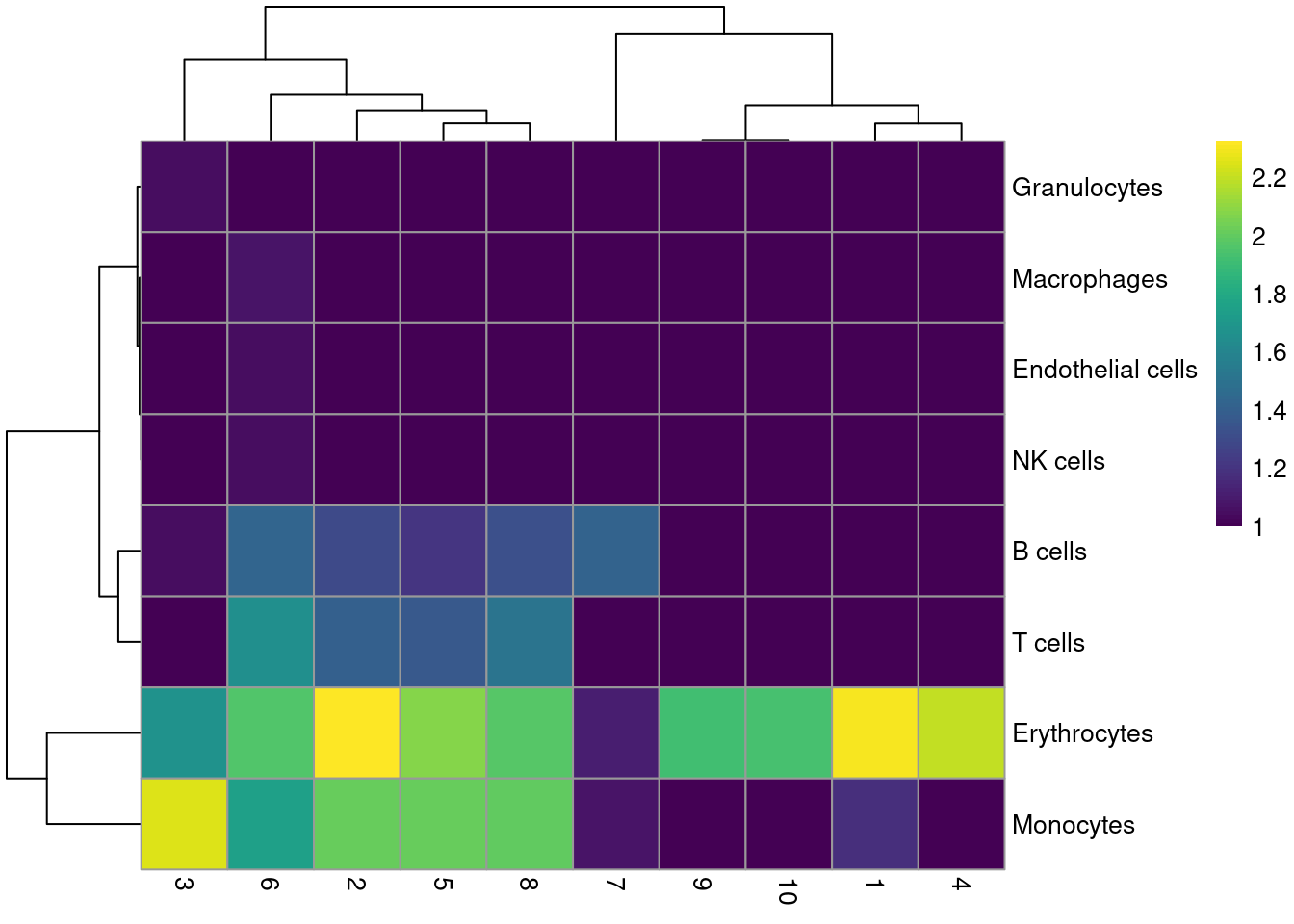
Figure 10.6: Heatmap of the distribution of cells for each cluster in the Nestorowa HSC dataset, based on their assignment to each label in the mouse RNA-seq references from the SingleR package.
10.10 Miscellaneous analyses
This dataset also contains information about the protein abundances in each cell from FACS. There is barely any heterogeneity in the chosen markers across the clusters (Figure 10.7); this is perhaps unsurprising given that all cells should be HSCs of some sort.
Y <- assay(altExp(sce.nest, "FACS"))
keep <- colSums(is.na(Y))==0 # Removing NA intensities.

se.averaged <- sumCountsAcrossCells(Y[,keep],
    colLabels(sce.nest)[keep], average=TRUE)
averaged <- assay(se.averaged)

log.intensities <- log2(averaged+1)
centered <- log.intensities - rowMeans(log.intensities)
pheatmap(centered, breaks=seq(-1, 1, length.out=101))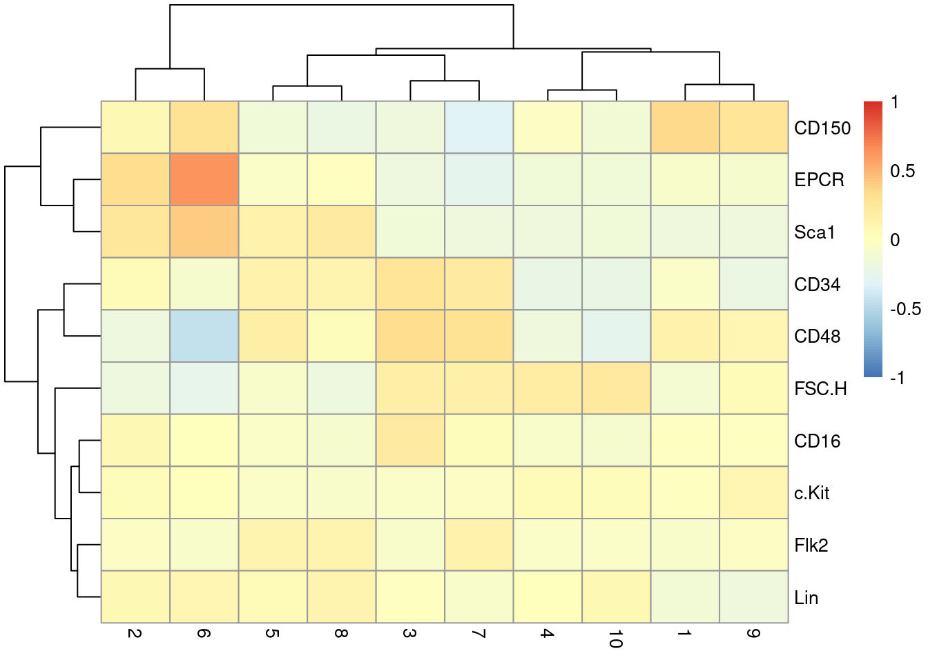
Figure 10.7: Heatmap of the centered log-average intensity for each target protein quantified by FACS in the Nestorowa HSC dataset.
Session Info
R version 4.4.0 beta (2024-04-15 r86425)
Platform: x86_64-pc-linux-gnu
Running under: Ubuntu 22.04.4 LTS

Matrix products: default
BLAS:   /home/biocbuild/bbs-3.19-bioc/R/lib/libRblas.so
LAPACK: /usr/lib/x86_64-linux-gnu/lapack/liblapack.so.3.10.0

locale:
 [1] LC_CTYPE=en_US.UTF-8       LC_NUMERIC=C
 [3] LC_TIME=en_GB              LC_COLLATE=C
 [5] LC_MONETARY=en_US.UTF-8    LC_MESSAGES=en_US.UTF-8
 [7] LC_PAPER=en_US.UTF-8       LC_NAME=C
 [9] LC_ADDRESS=C               LC_TELEPHONE=C
[11] LC_MEASUREMENT=en_US.UTF-8 LC_IDENTIFICATION=C

time zone: America/New_York
tzcode source: system (glibc)

attached base packages:
[1] stats4    stats     graphics  grDevices utils     datasets  methods
[8] base

other attached packages:
 [1] SingleR_2.6.0               pheatmap_1.0.12
 [3] scran_1.32.0                scater_1.32.0
 [5] ggplot2_3.5.1               scuttle_1.14.0
 [7] AnnotationHub_3.12.0        BiocFileCache_2.12.0
 [9] dbplyr_2.5.0                ensembldb_2.28.0
[11] AnnotationFilter_1.28.0     GenomicFeatures_1.56.0
[13] AnnotationDbi_1.66.0        scRNAseq_2.18.0
[15] SingleCellExperiment_1.26.0 SummarizedExperiment_1.34.0
[17] Biobase_2.64.0              GenomicRanges_1.56.0
[19] GenomeInfoDb_1.40.0         IRanges_2.38.0
[21] S4Vectors_0.42.0            BiocGenerics_0.50.0
[23] MatrixGenerics_1.16.0       matrixStats_1.3.0
[25] BiocStyle_2.32.0            rebook_1.14.0

loaded via a namespace (and not attached):
  [1] BiocIO_1.14.0             bitops_1.0-7
  [3] filelock_1.0.3            tibble_3.2.1
  [5] CodeDepends_0.6.6         graph_1.82.0
  [7] XML_3.99-0.16.1           lifecycle_1.0.4
  [9] httr2_1.0.1               edgeR_4.2.0
 [11] lattice_0.22-6            alabaster.base_1.4.0
 [13] magrittr_2.0.3            limma_3.60.0
 [15] sass_0.4.9                rmarkdown_2.26
 [17] jquerylib_0.1.4           yaml_2.3.8
 [19] metapod_1.12.0            cowplot_1.1.3
 [21] DBI_1.2.2                 RColorBrewer_1.1-3
 [23] abind_1.4-5               zlibbioc_1.50.0
 [25] Rtsne_0.17                purrr_1.0.2
 [27] RCurl_1.98-1.14           rappdirs_0.3.3
 [29] GenomeInfoDbData_1.2.12   ggrepel_0.9.5
 [31] irlba_2.3.5.1             alabaster.sce_1.4.0
 [33] dqrng_0.3.2               DelayedMatrixStats_1.26.0
 [35] codetools_0.2-20          DelayedArray_0.30.0
 [37] tidyselect_1.2.1          UCSC.utils_1.0.0
 [39] farver_2.1.1              ScaledMatrix_1.12.0
 [41] viridis_0.6.5             GenomicAlignments_1.40.0
 [43] jsonlite_1.8.8            BiocNeighbors_1.22.0
 [45] tools_4.4.0               Rcpp_1.0.12
 [47] glue_1.7.0                gridExtra_2.3
 [49] SparseArray_1.4.0         xfun_0.43
 [51] dplyr_1.1.4               HDF5Array_1.32.0
 [53] gypsum_1.0.0              withr_3.0.0
 [55] BiocManager_1.30.22       fastmap_1.1.1
 [57] rhdf5filters_1.16.0       bluster_1.14.0
 [59] fansi_1.0.6               digest_0.6.35
 [61] rsvd_1.0.5                R6_2.5.1
 [63] mime_0.12                 colorspace_2.1-0
 [65] RSQLite_2.3.6             paws.storage_0.5.0
 [67] celldex_1.14.0            utf8_1.2.4
 [69] generics_0.1.3            rtracklayer_1.64.0
 [71] httr_1.4.7                S4Arrays_1.4.0
 [73] pkgconfig_2.0.3           gtable_0.3.5
 [75] blob_1.2.4                XVector_0.44.0
 [77] htmltools_0.5.8.1         bookdown_0.39
 [79] ProtGenerics_1.36.0       scales_1.3.0
 [81] alabaster.matrix_1.4.0    png_0.1-8
 [83] knitr_1.46                rjson_0.2.21
 [85] curl_5.2.1                cachem_1.0.8
 [87] rhdf5_2.48.0              BiocVersion_3.19.1
 [89] parallel_4.4.0            vipor_0.4.7
 [91] restfulr_0.0.15           pillar_1.9.0
 [93] grid_4.4.0                alabaster.schemas_1.4.0
 [95] vctrs_0.6.5               BiocSingular_1.20.0
 [97] beachmat_2.20.0           cluster_2.1.6
 [99] beeswarm_0.4.0            evaluate_0.23
[101] cli_3.6.2                 locfit_1.5-9.9
[103] compiler_4.4.0            Rsamtools_2.20.0
[105] rlang_1.1.3               crayon_1.5.2
[107] paws.common_0.7.2         labeling_0.4.3
[109] ggbeeswarm_0.7.2          alabaster.se_1.4.0
[111] viridisLite_0.4.2         BiocParallel_1.38.0
[113] munsell_0.5.1             Biostrings_2.72.0
[115] lazyeval_0.2.2            Matrix_1.7-0
[117] dir.expiry_1.12.0         ExperimentHub_2.12.0
[119] sparseMatrixStats_1.16.0  bit64_4.0.5
[121] Rhdf5lib_1.26.0           KEGGREST_1.44.0
[123] statmod_1.5.0             alabaster.ranges_1.4.0
[125] highr_0.10                igraph_2.0.3
[127] memoise_2.0.1             bslib_0.7.0
[129] bit_4.0.5
References
Nestorowa, S., F. K. Hamey, B. Pijuan Sala, E. Diamanti, M. Shepherd, E. Laurenti, N. K. Wilson, D. G. Kent, and B. Gottgens. 2016. “A single-cell resolution map of mouse hematopoietic stem and progenitor cell differentiation.” Blood 128 (8): 20–31.