Chapter 5 Grun human pancreas (CEL-seq2)
5.1 Introduction
This workflow performs an analysis of the Grun et al. (2016) CEL-seq2 dataset consisting of human pancreas cells from various donors.
5.2 Data loading
We convert to Ensembl identifiers, and we remove duplicated genes or genes without Ensembl IDs.
5.3 Quality control
This dataset lacks mitochondrial genes so we will do without them for quality control.
We compute the median and MAD while blocking on the donor;
for donors where the assumption of a majority of high-quality cells seems to be violated (Figure 5.1),
we compute an appropriate threshold using the other donors as specified in the subset= argument.
library(scater)
stats <- perCellQCMetrics(sce.grun)

qc <- quickPerCellQC(stats, percent_subsets="altexps_ERCC_percent",
    batch=sce.grun$donor,
    subset=sce.grun$donor %in% c("D17", "D7", "D2"))

sce.grun <- sce.grun[,!qc$discard]colData(unfiltered) <- cbind(colData(unfiltered), stats)
unfiltered$discard <- qc$discard
gridExtra::grid.arrange(
plotColData(unfiltered, x="donor", y="sum", colour_by="discard") +
scale_y_log10() + ggtitle("Total count"),
plotColData(unfiltered, x="donor", y="detected", colour_by="discard") +
scale_y_log10() + ggtitle("Detected features"),
plotColData(unfiltered, x="donor", y="altexps_ERCC_percent",
colour_by="discard") + ggtitle("ERCC percent"),
ncol=2
)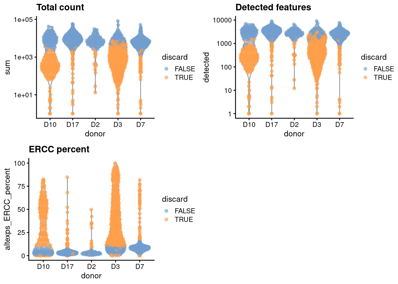
Figure 5.1: Distribution of each QC metric across cells from each donor of the Grun pancreas dataset. Each point represents a cell and is colored according to whether that cell was discarded.
##              low_lib_size            low_n_features high_altexps_ERCC_percent
##                       451                       510                       606
##                   discard
##                       664
5.4 Normalization
library(scran)
set.seed(1000) # for irlba.
clusters <- quickCluster(sce.grun)
sce.grun <- computeSumFactors(sce.grun, clusters=clusters)
sce.grun <- logNormCounts(sce.grun)## Min. 1st Qu. Median Mean 3rd Qu. Max.
## 0.098 0.508 0.791 1.000 1.230 10.072plot(librarySizeFactors(sce.grun), sizeFactors(sce.grun), pch=16,
xlab="Library size factors", ylab="Deconvolution factors", log="xy")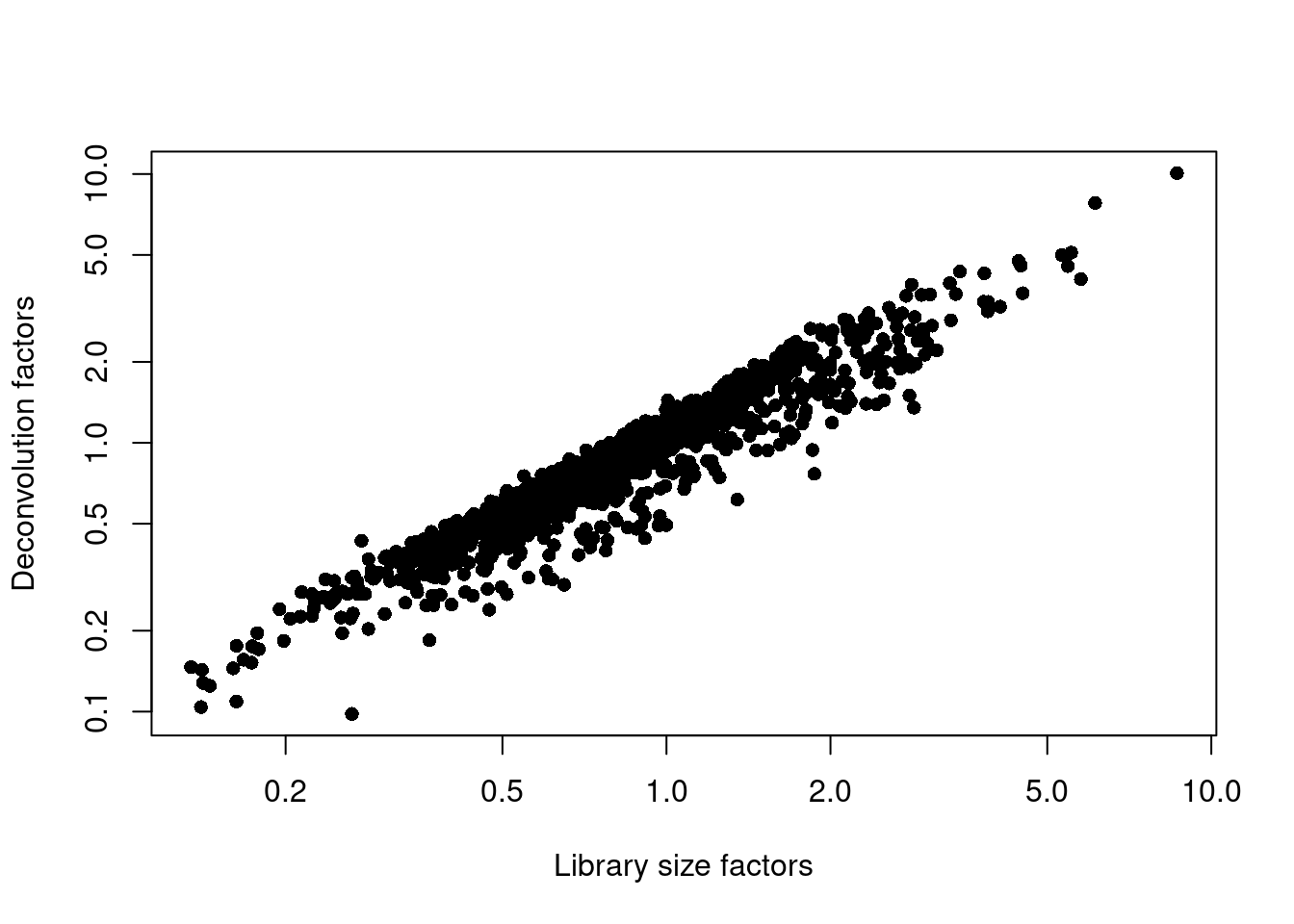
Figure 5.2: Relationship between the library size factors and the deconvolution size factors in the Grun pancreas dataset.
5.5 Variance modelling
We block on a combined plate and donor factor.
block <- paste0(sce.grun$sample, "_", sce.grun$donor)
dec.grun <- modelGeneVarWithSpikes(sce.grun, spikes="ERCC", block=block)
top.grun <- getTopHVGs(dec.grun, prop=0.1)
We examine the number of cells in each level of the blocking factor.
## block
##                  CD13+ sorted cells_D17       CD24+ CD44+ live sorted cells_D17
##                                      87                                      87
##                  CD63+ sorted cells_D10                TGFBR3+ sorted cells_D17
##                                      40                                      90
## exocrine fraction, live sorted cells_D2 exocrine fraction, live sorted cells_D3
##                                      82                                       7
##        live sorted cells, library 1_D10        live sorted cells, library 1_D17
##                                      33                                      88
##         live sorted cells, library 1_D3         live sorted cells, library 1_D7
##                                      25                                      85
##        live sorted cells, library 2_D10        live sorted cells, library 2_D17
##                                      35                                      83
##         live sorted cells, library 2_D3         live sorted cells, library 2_D7
##                                      27                                      84
##         live sorted cells, library 3_D3         live sorted cells, library 3_D7
##                                      16                                      83
##         live sorted cells, library 4_D3         live sorted cells, library 4_D7
## 29 83par(mfrow=c(6,3))
blocked.stats <- dec.grun$per.block
for (i in colnames(blocked.stats)) {
current <- blocked.stats[[i]]
plot(current$mean, current$total, main=i, pch=16, cex=0.5,
xlab="Mean of log-expression", ylab="Variance of log-expression")
curfit <- metadata(current)
points(curfit$mean, curfit$var, col="red", pch=16)
curve(curfit$trend(x), col='dodgerblue', add=TRUE, lwd=2)
}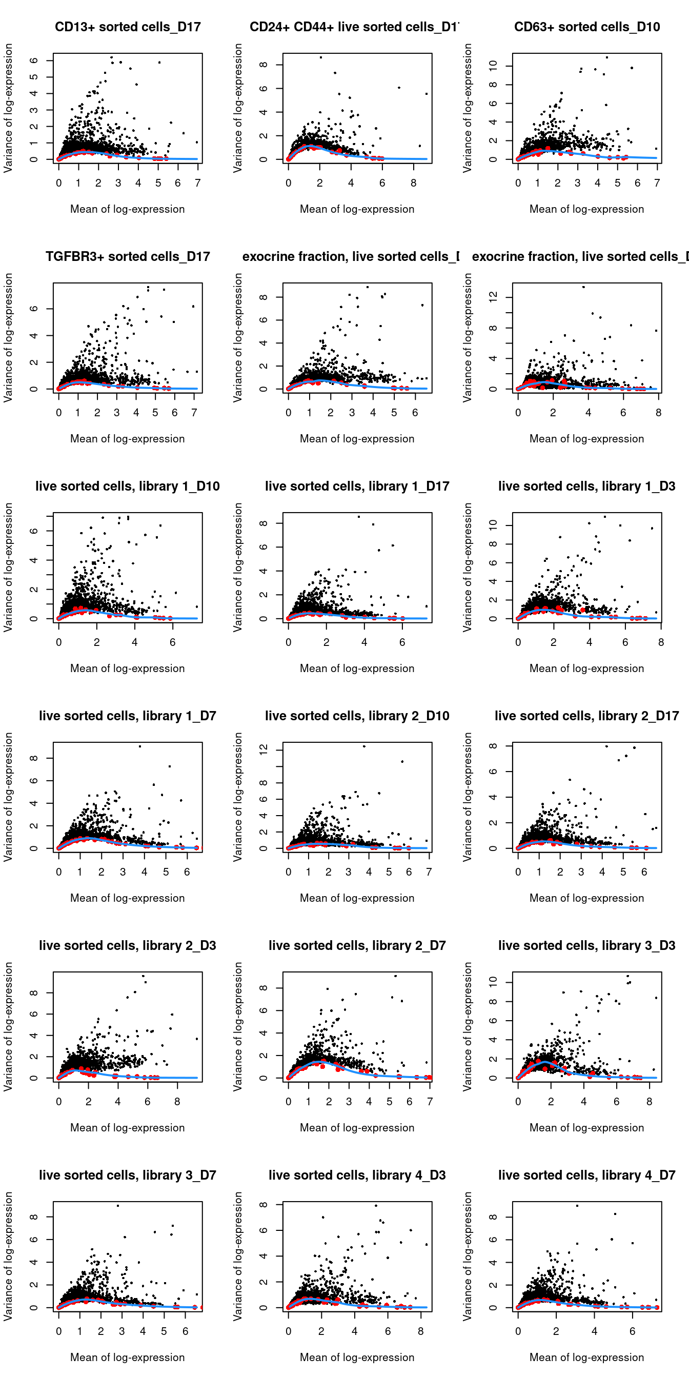
Figure 1.4: Per-gene variance as a function of the mean for the log-expression values in the Grun pancreas dataset. Each point represents a gene (black) with the mean-variance trend (blue) fitted to the spike-in transcripts (red) separately for each donor.
5.6 Data integration
library(batchelor)
set.seed(1001010)
merged.grun <- fastMNN(sce.grun, subset.row=top.grun, batch=sce.grun$donor)## D10 D17 D2 D3 D7
## [1,] 0.030046 0.03098 0.000000 0.00000 0.00000
## [2,] 0.007559 0.01196 0.038754 0.00000 0.00000
## [3,] 0.004060 0.00524 0.008091 0.05278 0.00000
## [4,] 0.013901 0.01682 0.017032 0.01576 0.055015.8 Clustering
snn.gr <- buildSNNGraph(merged.grun, use.dimred="corrected")
colLabels(merged.grun) <- factor(igraph::cluster_walktrap(snn.gr)$membership)## Donor
## Cluster D10 D17 D2 D3 D7
## 1 17 74 3 2 77
## 2 6 11 5 7 9
## 3 27 107 43 13 115
## 4 12 128 0 0 62
## 5 32 71 31 80 28
## 6 5 14 0 0 10
## 7 4 13 0 0 1
## 8 5 17 0 2 33gridExtra::grid.arrange(
plotTSNE(merged.grun, colour_by="label"),
plotTSNE(merged.grun, colour_by="batch"),
ncol=2
)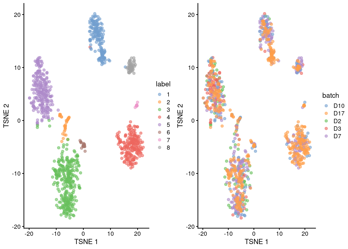
Figure 5.3: Obligatory \(t\)-SNE plots of the Grun pancreas dataset. Each point represents a cell that is colored by cluster (left) or batch (right).
Session Info
R version 4.4.0 beta (2024-04-15 r86425)
Platform: x86_64-pc-linux-gnu
Running under: Ubuntu 22.04.4 LTS

Matrix products: default
BLAS:   /home/biocbuild/bbs-3.19-bioc/R/lib/libRblas.so
LAPACK: /usr/lib/x86_64-linux-gnu/lapack/liblapack.so.3.10.0

locale:
 [1] LC_CTYPE=en_US.UTF-8       LC_NUMERIC=C
 [3] LC_TIME=en_GB              LC_COLLATE=C
 [5] LC_MONETARY=en_US.UTF-8    LC_MESSAGES=en_US.UTF-8
 [7] LC_PAPER=en_US.UTF-8       LC_NAME=C
 [9] LC_ADDRESS=C               LC_TELEPHONE=C
[11] LC_MEASUREMENT=en_US.UTF-8 LC_IDENTIFICATION=C

time zone: America/New_York
tzcode source: system (glibc)

attached base packages:
[1] stats4    stats     graphics  grDevices utils     datasets  methods
[8] base

other attached packages:
 [1] batchelor_1.20.0            scran_1.32.0
 [3] scater_1.32.0               ggplot2_3.5.1
 [5] scuttle_1.14.0              org.Hs.eg.db_3.19.1
 [7] AnnotationDbi_1.66.0        scRNAseq_2.18.0
 [9] SingleCellExperiment_1.26.0 SummarizedExperiment_1.34.0
[11] Biobase_2.64.0              GenomicRanges_1.56.0
[13] GenomeInfoDb_1.40.0         IRanges_2.38.0
[15] S4Vectors_0.42.0            BiocGenerics_0.50.0
[17] MatrixGenerics_1.16.0       matrixStats_1.3.0
[19] BiocStyle_2.32.0            rebook_1.14.0

loaded via a namespace (and not attached):
  [1] jsonlite_1.8.8            CodeDepends_0.6.6
  [3] magrittr_2.0.3            ggbeeswarm_0.7.2
  [5] GenomicFeatures_1.56.0    gypsum_1.0.0
  [7] farver_2.1.1              rmarkdown_2.26
  [9] BiocIO_1.14.0             zlibbioc_1.50.0
 [11] vctrs_0.6.5               memoise_2.0.1
 [13] Rsamtools_2.20.0          DelayedMatrixStats_1.26.0
 [15] RCurl_1.98-1.14           htmltools_0.5.8.1
 [17] S4Arrays_1.4.0            AnnotationHub_3.12.0
 [19] curl_5.2.1                BiocNeighbors_1.22.0
 [21] Rhdf5lib_1.26.0           SparseArray_1.4.0
 [23] rhdf5_2.48.0              sass_0.4.9
 [25] alabaster.base_1.4.0      bslib_0.7.0
 [27] alabaster.sce_1.4.0       httr2_1.0.1
 [29] cachem_1.0.8              ResidualMatrix_1.14.0
 [31] GenomicAlignments_1.40.0  igraph_2.0.3
 [33] lifecycle_1.0.4           pkgconfig_2.0.3
 [35] rsvd_1.0.5                Matrix_1.7-0
 [37] R6_2.5.1                  fastmap_1.1.1
 [39] GenomeInfoDbData_1.2.12   digest_0.6.35
 [41] colorspace_2.1-0          paws.storage_0.5.0
 [43] dqrng_0.3.2               irlba_2.3.5.1
 [45] ExperimentHub_2.12.0      RSQLite_2.3.6
 [47] beachmat_2.20.0           labeling_0.4.3
 [49] filelock_1.0.3            fansi_1.0.6
 [51] httr_1.4.7                abind_1.4-5
 [53] compiler_4.4.0            bit64_4.0.5
 [55] withr_3.0.0               BiocParallel_1.38.0
 [57] viridis_0.6.5             DBI_1.2.2
 [59] highr_0.10                HDF5Array_1.32.0
 [61] alabaster.ranges_1.4.0    alabaster.schemas_1.4.0
 [63] rappdirs_0.3.3            DelayedArray_0.30.0
 [65] bluster_1.14.0            rjson_0.2.21
 [67] tools_4.4.0               vipor_0.4.7
 [69] beeswarm_0.4.0            glue_1.7.0
 [71] restfulr_0.0.15           rhdf5filters_1.16.0
 [73] grid_4.4.0                Rtsne_0.17
 [75] cluster_2.1.6             generics_0.1.3
 [77] gtable_0.3.5              ensembldb_2.28.0
 [79] metapod_1.12.0            ScaledMatrix_1.12.0
 [81] BiocSingular_1.20.0       utf8_1.2.4
 [83] XVector_0.44.0            ggrepel_0.9.5
 [85] BiocVersion_3.19.1        pillar_1.9.0
 [87] limma_3.60.0              dplyr_1.1.4
 [89] BiocFileCache_2.12.0      lattice_0.22-6
 [91] rtracklayer_1.64.0        bit_4.0.5
 [93] tidyselect_1.2.1          paws.common_0.7.2
 [95] locfit_1.5-9.9            Biostrings_2.72.0
 [97] knitr_1.46                gridExtra_2.3
 [99] bookdown_0.39             ProtGenerics_1.36.0
[101] edgeR_4.2.0               xfun_0.43
[103] statmod_1.5.0             UCSC.utils_1.0.0
[105] lazyeval_0.2.2            yaml_2.3.8
[107] evaluate_0.23             codetools_0.2-20
[109] tibble_3.2.1              alabaster.matrix_1.4.0
[111] BiocManager_1.30.22       graph_1.82.0
[113] cli_3.6.2                 munsell_0.5.1
[115] jquerylib_0.1.4           Rcpp_1.0.12
[117] dir.expiry_1.12.0         dbplyr_2.5.0
[119] png_0.1-8                 XML_3.99-0.16.1
[121] parallel_4.4.0            blob_1.2.4
[123] AnnotationFilter_1.28.0   sparseMatrixStats_1.16.0
[125] bitops_1.0-7              viridisLite_0.4.2
[127] alabaster.se_1.4.0        scales_1.3.0
[129] crayon_1.5.2              rlang_1.1.3
[131] cowplot_1.1.3             KEGGREST_1.44.0
References
Grun, D., M. J. Muraro, J. C. Boisset, K. Wiebrands, A. Lyubimova, G. Dharmadhikari, M. van den Born, et al. 2016. “De Novo Prediction of Stem Cell Identity using Single-Cell Transcriptome Data.” Cell Stem Cell 19 (2): 266–77.