Chapter 3 Feature selection, redux
3.1 Overview
Basic Chapter 3 introduced the principles and methodology for feature selection in scRNA-seq data.
This chapter provides some commentary on some additional options at each step,
including the fine-tuning of the fitted trend in modelGeneVar(),
how to handle more uninteresting factors of variation with linear models,
and the use of coefficient of variation to quantify variation.
We also got through a number of other HVG selection strategies that may be of use.
3.2 Fine-tuning the fitted trend
The trend fit has several useful parameters (see ?fitTrendVar) that can be tuned for a more appropriate fit.
For example, the defaults can occasionally yield an overfitted trend when the few high-abundance genes are also highly variable.
In such cases, users can reduce the contribution of those high-abundance genes by turning off density weights,
as demonstrated in Figure 3.1 with a single donor from the Segerstolpe et al. (2016) dataset.
#--- loading ---#
library(scRNAseq)
sce.seger <- SegerstolpePancreasData()

#--- gene-annotation ---#
library(AnnotationHub)
edb <- AnnotationHub()[["AH73881"]]
symbols <- rowData(sce.seger)$symbol
ens.id <- mapIds(edb, keys=symbols, keytype="SYMBOL", column="GENEID")
ens.id <- ifelse(is.na(ens.id), symbols, ens.id)

# Removing duplicated rows.
keep <- !duplicated(ens.id)
sce.seger <- sce.seger[keep,]
rownames(sce.seger) <- ens.id[keep]

#--- sample-annotation ---#
emtab.meta <- colData(sce.seger)[,c("cell type", "disease",
    "individual", "single cell well quality")]
colnames(emtab.meta) <- c("CellType", "Disease", "Donor", "Quality")
colData(sce.seger) <- emtab.meta

sce.seger$CellType <- gsub(" cell", "", sce.seger$CellType)
sce.seger$CellType <- paste0(
    toupper(substr(sce.seger$CellType, 1, 1)),
    substring(sce.seger$CellType, 2))

#--- quality-control ---#
low.qual <- sce.seger$Quality == "low quality cell"

library(scater)
stats <- perCellQCMetrics(sce.seger)
qc <- quickPerCellQC(stats, percent_subsets="altexps_ERCC_percent",
    batch=sce.seger$Donor,
    subset=!sce.seger$Donor %in% c("HP1504901", "HP1509101"))

sce.seger <- sce.seger[,!(qc$discard | low.qual)]

#--- normalization ---#
library(scran)
clusters <- quickCluster(sce.seger)
sce.seger <- computeSumFactors(sce.seger, clusters=clusters)
sce.seger <- logNormCounts(sce.seger) library(scran)
sce.seger <- sce.seger[,sce.seger$Donor=="HP1507101"]
dec.default <- modelGeneVar(sce.seger)
dec.noweight <- modelGeneVar(sce.seger, density.weights=FALSE)
fit.default <- metadata(dec.default)
plot(fit.default$mean, fit.default$var, xlab="Mean of log-expression",
ylab="Variance of log-expression")
curve(fit.default$trend(x), col="dodgerblue", add=TRUE, lwd=2)
fit.noweight <- metadata(dec.noweight)
curve(fit.noweight$trend(x), col="red", add=TRUE, lwd=2)
legend("topleft", col=c("dodgerblue", "red"), legend=c("Default", "No weight"), lwd=2)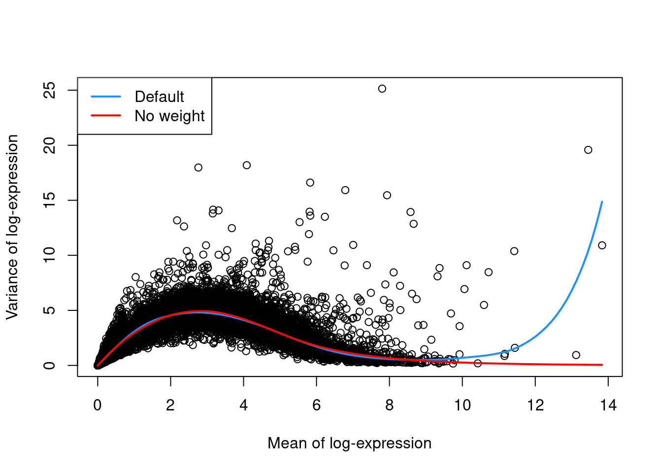
Figure 3.1: Variance in the Segerstolpe pancreas data set as a function of the mean. Each point represents a gene while the lines represent the trend fitted to all genes with default parameters (blue) or without weights (red).
3.3 Handling covariates with linear models
For experiments with multiple batches, the use of block-specific trends with block= in modelGeneVar() is the recommended approach for avoiding unwanted variation.
However, this is not possible for experimental designs involving multiple unwanted factors of variation and/or continuous covariates.
In such cases, we can use the design= argument to specify a design matrix with uninteresting factors of variation.
This fits a linear model to the expression values for each gene to obtain the residual variance.
We illustrate again with the 416B data set, blocking on the plate of origin and oncogene induction.
(The same argument is available in modelGeneVar() when spike-ins are not available.)
#--- loading ---#
library(scRNAseq)
sce.416b <- LunSpikeInData(which="416b")
sce.416b$block <- factor(sce.416b$block)

#--- gene-annotation ---#
library(AnnotationHub)
ens.mm.v97 <- AnnotationHub()[["AH73905"]]
rowData(sce.416b)$ENSEMBL <- rownames(sce.416b)
rowData(sce.416b)$SYMBOL <- mapIds(ens.mm.v97, keys=rownames(sce.416b),
    keytype="GENEID", column="SYMBOL")
rowData(sce.416b)$SEQNAME <- mapIds(ens.mm.v97, keys=rownames(sce.416b),
    keytype="GENEID", column="SEQNAME")

library(scater)
rownames(sce.416b) <- uniquifyFeatureNames(rowData(sce.416b)$ENSEMBL,
    rowData(sce.416b)$SYMBOL)

#--- quality-control ---#
mito <- which(rowData(sce.416b)$SEQNAME=="MT")
stats <- perCellQCMetrics(sce.416b, subsets=list(Mt=mito))
qc <- quickPerCellQC(stats, percent_subsets=c("subsets_Mt_percent",
    "altexps_ERCC_percent"), batch=sce.416b$block)
sce.416b <- sce.416b[,!qc$discard]

#--- normalization ---#
library(scran)
sce.416b <- computeSumFactors(sce.416b)
sce.416b <- logNormCounts(sce.416b)
design <- model.matrix(~factor(block) + phenotype, colData(sce.416b))
dec.design.416b <- modelGeneVarWithSpikes(sce.416b, "ERCC", design=design)
dec.design.416b[order(dec.design.416b$bio, decreasing=TRUE),]## DataFrame with 46604 rows and 6 columns
## mean total tech bio p.value FDR
## <numeric> <numeric> <numeric> <numeric> <numeric> <numeric>
## Lyz2 6.61097 8.90513 1.50405 7.40107 1.78185e-172 1.28493e-169
## Ccnb2 5.97776 9.54373 2.24180 7.30192 7.77223e-77 1.44497e-74
## Gem 5.90225 9.54358 2.35175 7.19183 5.49587e-68 8.12330e-66
## Cenpa 5.81349 8.65622 2.48792 6.16830 2.08035e-45 1.52796e-43
## Idh1 5.99343 8.32113 2.21965 6.10148 2.42819e-55 2.41772e-53
## ... ... ... ... ... ... ...
## Gm5054 2.90434 0.463698 6.77000 -6.30630 1 1
## Gm12191 3.55920 0.170709 6.53285 -6.36214 1 1
## Gm7429 3.45394 0.248351 6.63458 -6.38623 1 1
## Gm16378 2.83987 0.208215 6.74663 -6.53841 1 1
## Rps2-ps2 3.11324 0.202307 6.78484 -6.58253 1 1This strategy is simple but somewhat inaccurate as it does not consider the mean expression in each blocking level.
To illustrate, assume we have an experiment with two equally-sized batches where the mean-variance trend in each batch is the same as that observed in Figure 3.1.
Imagine that we have two genes with variances lying on this trend;
the first gene has an average expression of 0 in one batch and 6 in the other batch,
while the second gene with an average expression of 3 in both batches.
Both genes would have the same mean across all cells but quite different variances, making it difficult to fit a single mean-variance trend - despite both genes following the mean-variance trend in each of their respective batches!
The block= approach is safer as it handles the trend fitting and decomposition within each batch, and should be preferred in all situations where it is applicable.
3.4 Using the coefficient of variation
An alternative approach to quantification uses the squared coefficient of variation (CV2) of the normalized expression values prior to log-transformation.
The CV2 is a widely used metric for describing variation in non-negative data and is closely related to the dispersion parameter of the negative binomial distribution in packages like edgeR and DESeq2.
We compute the CV2 for each gene in the PBMC dataset using the modelGeneCV2() function, which provides a robust implementation of the approach described by Brennecke et al. (2013).
#--- loading ---#
library(DropletTestFiles)
raw.path <- getTestFile("tenx-2.1.0-pbmc4k/1.0.0/raw.tar.gz")
out.path <- file.path(tempdir(), "pbmc4k")
untar(raw.path, exdir=out.path)

library(DropletUtils)
fname <- file.path(out.path, "raw_gene_bc_matrices/GRCh38")
sce.pbmc <- read10xCounts(fname, col.names=TRUE)

#--- gene-annotation ---#
library(scater)
rownames(sce.pbmc) <- uniquifyFeatureNames(
    rowData(sce.pbmc)$ID, rowData(sce.pbmc)$Symbol)

library(EnsDb.Hsapiens.v86)
location <- mapIds(EnsDb.Hsapiens.v86, keys=rowData(sce.pbmc)$ID,
    column="SEQNAME", keytype="GENEID")

#--- cell-detection ---#
set.seed(100)
e.out <- emptyDrops(counts(sce.pbmc))
sce.pbmc <- sce.pbmc[,which(e.out$FDR <= 0.001)]

#--- quality-control ---#
stats <- perCellQCMetrics(sce.pbmc, subsets=list(Mito=which(location=="MT")))
high.mito <- isOutlier(stats$subsets_Mito_percent, type="higher")
sce.pbmc <- sce.pbmc[,!high.mito]

#--- normalization ---#
library(scran)
set.seed(1000)
clusters <- quickCluster(sce.pbmc)
sce.pbmc <- computeSumFactors(sce.pbmc, cluster=clusters)
sce.pbmc <- logNormCounts(sce.pbmc)This allows us to model the mean-variance relationship when considering the relevance of each gene (Figure 3.2).
Again, our assumption is that most genes contain random noise and that the trend captures mostly technical variation.
Large CV2 values that deviate strongly from the trend are likely to represent genes affected by biological structure.
If spike-ins are available, we can also fit the trend to the spike-ins via the modelGeneCV2WithSpikes() function.
fit.cv2.pbmc <- metadata(dec.cv2.pbmc)
plot(fit.cv2.pbmc$mean, fit.cv2.pbmc$cv2, log="xy")
curve(fit.cv2.pbmc$trend(x), col="dodgerblue", add=TRUE, lwd=2)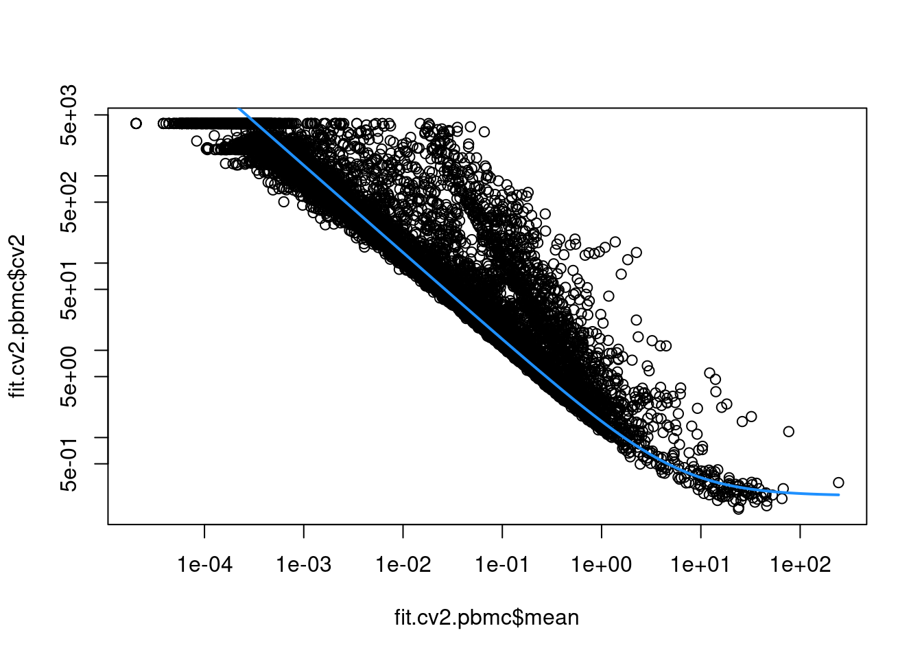
Figure 3.2: CV2 in the PBMC data set as a function of the mean. Each point represents a gene while the blue line represents the fitted trend.
For each gene, we quantify the deviation from the trend in terms of the ratio of its CV2 to the fitted value of trend at its abundance. This is more appropriate than the directly subtracting the trend from the CV2, as the magnitude of the ratio is not affected by the mean.
## DataFrame with 33694 rows and 6 columns
##                 mean     total     trend     ratio   p.value       FDR
##            <numeric> <numeric> <numeric> <numeric> <numeric> <numeric>
## PPBP       2.2437397   132.364  0.803689   164.696         0         0
## PRTFDC1    0.0658743  3197.564 20.266829   157.773         0         0
## HIST1H2AC  1.3731487   175.035  1.176934   148.721         0         0
## FAM81B     0.0477082  3654.419 27.902078   130.973         0         0
## PF4        1.8333127   109.451  0.935484   116.999         0         0
## ...              ...       ...       ...       ...       ...       ...
## AC023491.2         0       NaN       Inf       NaN       NaN       NaN
## AC233755.2         0       NaN       Inf       NaN       NaN       NaN
## AC233755.1         0       NaN       Inf       NaN       NaN       NaN
## AC213203.1         0       NaN       Inf       NaN       NaN       NaN
## FAM231B            0       NaN       Inf       NaN       NaN       NaN
We can then select HVGs based on the largest ratios using getTopHVGs().
## chr [1:1000] "PPBP" "PRTFDC1" "HIST1H2AC" "FAM81B" "PF4" "GNG11" ...Both the CV2 and the variance of log-counts are effective metrics for quantifying variation in gene expression. The CV2 tends to give higher rank to low-abundance HVGs driven by upregulation in rare subpopulations, for which the increase in variance on the raw scale is stronger than that on the log-scale. However, the variation described by the CV2 is less directly relevant to downstream procedures operating on the log-counts, and the reliance on the ratio can assign high rank to uninteresting genes with low absolute variance. As such, we prefer to use the variance of log-counts for feature selection, though many of the same principles apply to procedures based on the CV2.
3.5 More HVG selection strategies
3.5.1 Keeping all genes above the trend
Here, the aim is to only remove the obviously uninteresting genes with variances below the trend.
By doing so, we avoid the need to make any judgement calls regarding what level of variation is interesting enough to retain.
This approach represents one extreme of the bias-variance trade-off where bias is minimized at the cost of maximizing noise.
For modelGeneVar(), it equates to keeping all positive biological components:
dec.pbmc <- modelGeneVar(sce.pbmc)
hvg.pbmc.var.3 <- getTopHVGs(dec.pbmc, var.threshold=0)
length(hvg.pbmc.var.3)
## [1] 12745For modelGeneCV2(), this involves keeping all ratios above 1:
hvg.pbmc.cv2.3 <- getTopHVGs(dec.cv2.pbmc, var.field="ratio", var.threshold=1)
length(hvg.pbmc.cv2.3)
## [1] 6643By retaining all potential biological signal, we give secondary population structure the chance to manifest. This is most useful for rare subpopulations where the relevant markers will not exhibit strong overdispersion owing to the small number of affected cells. It will also preserve a weak but consistent effect across many genes with small biological components; admittedly, though, this is not of major interest in most scRNA-seq studies given the difficulty of experimentally validating population structure in the absence of strong marker genes.
The obvious cost is that more noise is also captured, which can reduce the resolution of otherwise well-separated populations and mask the secondary signal that we were trying to preserve. The use of more genes also introduces more computational work in each downstream step. This strategy is thus best suited to very heterogeneous populations containing many different cell types (possibly across many datasets that are to be merged, as in Multi-sample Chapter 1) where there is a justified fear of ignoring marker genes for low-abundance subpopulations under a competitive top \(X\) approach.
3.5.2 Based on significance
Another approach to feature selection is to set a fixed threshold of one of the metrics. This is most commonly done with the (adjusted) \(p\)-value reported by each of the above methods. The \(p\)-value for each gene is generated by testing against the null hypothesis that the variance is equal to the trend. For example, we might define our HVGs as all genes that have adjusted \(p\)-values below 0.05.
## [1] 813This approach is simple to implement and - if the test holds its size - it controls the false discovery rate (FDR). That is, it returns a subset of genes where the proportion of false positives is expected to be below the specified threshold. This can occasionally be useful in applications where the HVGs themselves are of interest. For example, if we were to use the list of HVGs in further experiments to verify the existence of heterogeneous expression for some of the genes, we would want to control the FDR in that list.
The downside of this approach is that it is less predictable than the top \(X\) strategy. The number of genes returned depends on the type II error rate of the test and the severity of the multiple testing correction. One might obtain no genes or every gene at a given FDR threshold, depending on the circumstances. Moreover, control of the FDR is usually not helpful at this stage of the analysis. We are not interpreting the individual HVGs themselves but are only using them for feature selection prior to downstream steps. There is no reason to think that a 5% threshold on the FDR yields a more suitable compromise between bias and noise compared to the top \(X\) selection.
As an aside, we might consider ranking genes by the \(p\)-value instead of the biological component for use in a top \(X\) approach. This results in some counterintuitive behavior due to the nature of the underlying hypothesis test, which is based on the ratio of the total variance to the expected technical variance. Ranking based on \(p\)-value tends to prioritize HVGs that are more likely to be true positives but, at the same time, less likely to be biologically interesting. Many of the largest ratios are observed in high-abundance genes and are driven by very low technical variance; the total variance is typically modest for such genes, and they do not contribute much to population heterogeneity in absolute terms. (Note that the same can be said of the ratio of CV2 values, as briefly discussed above.)
3.5.3 Selecting a priori genes of interest
A blunt yet effective feature selection strategy is to use pre-defined sets of interesting genes. The aim is to focus on specific aspects of biological heterogeneity that may be masked by other factors when using unsupervised methods for HVG selection. One example application lies in the dissection of transcriptional changes during the earliest stages of cell fate commitment (Messmer et al. 2019), which may be modest relative to activity in other pathways (e.g., cell cycle, metabolism). Indeed, if our aim is to show that there is no meaningful heterogeneity in a given pathway, we would - at the very least - be obliged to repeat our analysis using only the genes in that pathway to maximize power for detecting such heterogeneity.
Using scRNA-seq data in this manner is conceptually equivalent to a fluorescence activated cell sorting (FACS) experiment, with the convenience of being able to (re)define the features of interest at any time. For example, in the PBMC dataset, we might use some of the C7 immunologic signatures from MSigDB (Godec et al. 2016) to improve resolution of the various T cell subtypes. We stress that there is no shame in leveraging prior biological knowledge to address specific hypotheses in this manner. We say this because a common refrain in genomics is that the data analysis should be “unbiased”, i.e., free from any biological preconceptions. This is admirable but such “biases” are already present at every stage, starting with experimental design and ending with the interpretation of the data.
library(msigdbr)
c7.sets <- msigdbr(species = "Homo sapiens", category = "C7")
head(unique(c7.sets$gs_name))
## [1] "ANDERSON_BLOOD_CN54GP140_ADJUVANTED_WITH_GLA_AF_AGE_18_45YO_1DY_DN"
## [2] "ANDERSON_BLOOD_CN54GP140_ADJUVANTED_WITH_GLA_AF_AGE_18_45YO_1DY_UP"
## [3] "ANDERSON_BLOOD_CN54GP140_ADJUVANTED_WITH_GLA_AF_AGE_18_45YO_3DY_DN"
## [4] "ANDERSON_BLOOD_CN54GP140_ADJUVANTED_WITH_GLA_AF_AGE_18_45YO_3DY_UP"
## [5] "ANDERSON_BLOOD_CN54GP140_ADJUVANTED_WITH_GLA_AF_AGE_18_45YO_6HR_DN"
## [6] "ANDERSON_BLOOD_CN54GP140_ADJUVANTED_WITH_GLA_AF_AGE_18_45YO_6HR_UP"# Using the Goldrath sets to distinguish CD8 subtypes
cd8.sets <- c7.sets[grep("GOLDRATH", c7.sets$gs_name),]
cd8.genes <- rowData(sce.pbmc)$Symbol %in% cd8.sets$human_gene_symbol
summary(cd8.genes)## Mode FALSE TRUE
## logical 32872 822# Using GSE11924 to distinguish between T helper subtypes
th.sets <- c7.sets[grep("GSE11924", c7.sets$gs_name),]
th.genes <- rowData(sce.pbmc)$Symbol %in% th.sets$human_gene_symbol
summary(th.genes)## Mode FALSE TRUE
## logical 31796 1898# Using GSE11961 to distinguish between B cell subtypes
b.sets <- c7.sets[grep("GSE11961", c7.sets$gs_name),]
b.genes <- rowData(sce.pbmc)$Symbol %in% b.sets$human_gene_symbol
summary(b.genes)## Mode FALSE TRUE
## logical 28211 5483Of course, the downside of focusing on pre-defined genes is that it will limit our capacity to detect novel or unexpected aspects of variation. Thus, this kind of focused analysis should be complementary to (rather than a replacement for) the unsupervised feature selection strategies discussed previously.
Alternatively, we can invert this reasoning to remove genes that are unlikely to be of interest prior to downstream analyses. This eliminates unwanted variation that could mask relevant biology and interfere with interpretation of the results. Ribosomal protein genes or mitochondrial genes are common candidates for removal, especially in situations with varying levels of cell damage within a population. For immune cell subsets, we might also be inclined to remove immunoglobulin genes and T cell receptor genes for which clonal expression introduces (possibly irrelevant) population structure.
# Identifying ribosomal proteins:
ribo.discard <- grepl("^RP[SL]\\d+", rownames(sce.pbmc))
sum(ribo.discard)
## [1] 99# A more curated approach for identifying ribosomal protein genes:
c2.sets <- msigdbr(species = "Homo sapiens", category = "C2")
ribo.set <- c2.sets[c2.sets$gs_name=="KEGG_RIBOSOME",]$human_gene_symbol
ribo.discard <- rownames(sce.pbmc) %in% ribo.set
sum(ribo.discard)## [1] 87library(AnnotationHub)
edb <- AnnotationHub()[["AH73881"]]
anno <- select(edb, keys=rowData(sce.pbmc)$ID, keytype="GENEID",
columns="TXBIOTYPE")
# Removing immunoglobulin variable chains:
igv.set <- anno$GENEID[anno$TXBIOTYPE %in% c("IG_V_gene", "IG_V_pseudogene")]
igv.discard <- rowData(sce.pbmc)$ID %in% igv.set
sum(igv.discard)## [1] 326# Removing TCR variable chains:
tcr.set <- anno$GENEID[anno$TXBIOTYPE %in% c("TR_V_gene", "TR_V_pseudogene")]
tcr.discard <- rowData(sce.pbmc)$ID %in% tcr.set
sum(tcr.discard)## [1] 138In practice, we tend to err on the side of caution and abstain from preemptive filtering on biological function until these genes are demonstrably problematic in downstream analyses.
Session Info
R version 4.2.2 (2022-10-31)
Platform: x86_64-pc-linux-gnu (64-bit)
Running under: Ubuntu 20.04.5 LTS

Matrix products: default
BLAS:   /home/biocbuild/bbs-3.16-bioc/R/lib/libRblas.so
LAPACK: /home/biocbuild/bbs-3.16-bioc/R/lib/libRlapack.so

locale:
 [1] LC_CTYPE=en_US.UTF-8       LC_NUMERIC=C
 [3] LC_TIME=en_GB              LC_COLLATE=C
 [5] LC_MONETARY=en_US.UTF-8    LC_MESSAGES=en_US.UTF-8
 [7] LC_PAPER=en_US.UTF-8       LC_NAME=C
 [9] LC_ADDRESS=C               LC_TELEPHONE=C
[11] LC_MEASUREMENT=en_US.UTF-8 LC_IDENTIFICATION=C

attached base packages:
[1] stats4    stats     graphics  grDevices utils     datasets  methods
[8] base

other attached packages:
 [1] ensembldb_2.22.0            AnnotationFilter_1.22.0
 [3] GenomicFeatures_1.50.4      AnnotationDbi_1.60.0
 [5] AnnotationHub_3.6.0         BiocFileCache_2.6.0
 [7] dbplyr_2.3.0                msigdbr_7.5.1
 [9] scran_1.26.2                scuttle_1.8.4
[11] SingleCellExperiment_1.20.0 SummarizedExperiment_1.28.0
[13] Biobase_2.58.0              GenomicRanges_1.50.2
[15] GenomeInfoDb_1.34.8         IRanges_2.32.0
[17] S4Vectors_0.36.1            BiocGenerics_0.44.0
[19] MatrixGenerics_1.10.0       matrixStats_0.63.0
[21] BiocStyle_2.26.0            rebook_1.8.0

loaded via a namespace (and not attached):
  [1] rjson_0.2.21                  ellipsis_0.3.2
  [3] bluster_1.8.0                 XVector_0.38.0
  [5] BiocNeighbors_1.16.0          bit64_4.0.5
  [7] interactiveDisplayBase_1.36.0 fansi_1.0.4
  [9] xml2_1.3.3                    codetools_0.2-18
 [11] sparseMatrixStats_1.10.0      cachem_1.0.6
 [13] knitr_1.42                    jsonlite_1.8.4
 [15] Rsamtools_2.14.0              cluster_2.1.4
 [17] png_0.1-8                     graph_1.76.0
 [19] shiny_1.7.4                   BiocManager_1.30.19
 [21] compiler_4.2.2                httr_1.4.4
 [23] dqrng_0.3.0                   lazyeval_0.2.2
 [25] assertthat_0.2.1              Matrix_1.5-3
 [27] fastmap_1.1.0                 limma_3.54.1
 [29] cli_3.6.0                     later_1.3.0
 [31] BiocSingular_1.14.0           prettyunits_1.1.1
 [33] htmltools_0.5.4               tools_4.2.2
 [35] rsvd_1.0.5                    igraph_1.3.5
 [37] glue_1.6.2                    GenomeInfoDbData_1.2.9
 [39] dplyr_1.1.0                   rappdirs_0.3.3
 [41] Rcpp_1.0.10                   jquerylib_0.1.4
 [43] vctrs_0.5.2                   Biostrings_2.66.0
 [45] babelgene_22.9                rtracklayer_1.58.0
 [47] DelayedMatrixStats_1.20.0     stringr_1.5.0
 [49] xfun_0.36                     beachmat_2.14.0
 [51] mime_0.12                     lifecycle_1.0.3
 [53] irlba_2.3.5.1                 restfulr_0.0.15
 [55] statmod_1.5.0                 XML_3.99-0.13
 [57] edgeR_3.40.2                  zlibbioc_1.44.0
 [59] ProtGenerics_1.30.0           hms_1.1.2
 [61] promises_1.2.0.1              parallel_4.2.2
 [63] yaml_2.3.7                    curl_5.0.0
 [65] memoise_2.0.1                 sass_0.4.5
 [67] biomaRt_2.54.0                stringi_1.7.12
 [69] RSQLite_2.2.20                BiocVersion_3.16.0
 [71] highr_0.10                    BiocIO_1.8.0
 [73] ScaledMatrix_1.6.0            filelock_1.0.2
 [75] BiocParallel_1.32.5           rlang_1.0.6
 [77] pkgconfig_2.0.3               bitops_1.0-7
 [79] evaluate_0.20                 lattice_0.20-45
 [81] purrr_1.0.1                   GenomicAlignments_1.34.0
 [83] CodeDepends_0.6.5             bit_4.0.5
 [85] tidyselect_1.2.0              magrittr_2.0.3
 [87] bookdown_0.32                 R6_2.5.1
 [89] generics_0.1.3                metapod_1.6.0
 [91] DelayedArray_0.24.0           DBI_1.1.3
 [93] pillar_1.8.1                  withr_2.5.0
 [95] KEGGREST_1.38.0               RCurl_1.98-1.10
 [97] tibble_3.1.8                  dir.expiry_1.6.0
 [99] crayon_1.5.2                  utf8_1.2.3
[101] rmarkdown_2.20                progress_1.2.2
[103] locfit_1.5-9.7                grid_4.2.2
[105] blob_1.2.3                    digest_0.6.31
[107] xtable_1.8-4                  httpuv_1.6.8
[109] bslib_0.4.2
References
Brennecke, P., S. Anders, J. K. Kim, A. A. Kołodziejczyk, X. Zhang, V. Proserpio, B. Baying, et al. 2013. “Accounting for technical noise in single-cell RNA-seq experiments.” Nat. Methods 10 (11): 1093–5.
Godec, J., Y. Tan, A. Liberzon, P. Tamayo, S. Bhattacharya, A. J. Butte, J. P. Mesirov, and W. N. Haining. 2016. “Compendium of Immune Signatures Identifies Conserved and Species-Specific Biology in Response to Inflammation.” Immunity 44 (1): 194–206.
Messmer, T., F. von Meyenn, A. Savino, F. Santos, H. Mohammed, A. T. L. Lun, J. C. Marioni, and W. Reik. 2019. “Transcriptional heterogeneity in naive and primed human pluripotent stem cells at single-cell resolution.” Cell Rep 26 (4): 815–24.
Segerstolpe, A., A. Palasantza, P. Eliasson, E. M. Andersson, A. C. Andreasson, X. Sun, S. Picelli, et al. 2016. “Single-Cell Transcriptome Profiling of Human Pancreatic Islets in Health and Type 2 Diabetes.” Cell Metab. 24 (4): 593–607.