Chapter 4 Dimensionality reduction, redux
4.1 Overview
Basic Chapter 4 introduced the key concepts for dimensionality reduction of scRNA-seq data. Here, we describe some data-driven strategies for picking an appropriate number of top PCs for downstream analyses. We also demonstrate some other dimensionality reduction strategies that operate on the raw counts. For the most part, we will be again using the Zeisel et al. (2015) dataset:
#--- loading ---#
library(scRNAseq)
sce.zeisel <- ZeiselBrainData()

library(scater)
sce.zeisel <- aggregateAcrossFeatures(sce.zeisel,
    id=sub("_loc[0-9]+$", "", rownames(sce.zeisel)))

#--- gene-annotation ---#
library(org.Mm.eg.db)
rowData(sce.zeisel)$Ensembl <- mapIds(org.Mm.eg.db,
    keys=rownames(sce.zeisel), keytype="SYMBOL", column="ENSEMBL")

#--- quality-control ---#
stats <- perCellQCMetrics(sce.zeisel, subsets=list(
    Mt=rowData(sce.zeisel)$featureType=="mito"))
qc <- quickPerCellQC(stats, percent_subsets=c("altexps_ERCC_percent",
    "subsets_Mt_percent"))
sce.zeisel <- sce.zeisel[,!qc$discard]

#--- normalization ---#
library(scran)
set.seed(1000)
clusters <- quickCluster(sce.zeisel)
sce.zeisel <- computeSumFactors(sce.zeisel, cluster=clusters)
sce.zeisel <- logNormCounts(sce.zeisel)

#--- variance-modelling ---#
dec.zeisel <- modelGeneVarWithSpikes(sce.zeisel, "ERCC")
top.hvgs <- getTopHVGs(dec.zeisel, prop=0.1)4.2 More choices for the number of PCs
4.2.1 Using the elbow point
A simple heuristic for choosing the suitable number of PCs \(d\) involves identifying the elbow point in the percentage of variance explained by successive PCs. This refers to the “elbow” in the curve of a scree plot as shown in Figure 4.1.
# Percentage of variance explained is tucked away in the attributes.
percent.var <- attr(reducedDim(sce.zeisel), "percentVar")

library(PCAtools)
chosen.elbow <- findElbowPoint(percent.var)
chosen.elbow
## [1] 7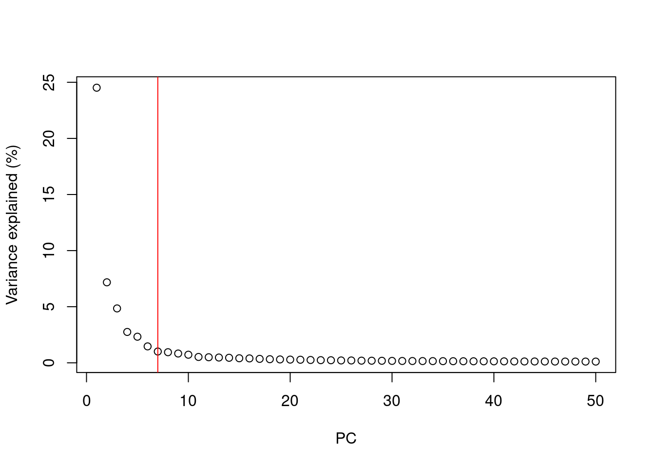
Figure 4.1: Percentage of variance explained by successive PCs in the Zeisel brain data. The identified elbow point is marked with a red line.
Our assumption is that each of the top PCs capturing biological signal should explain much more variance than the remaining PCs.
Thus, there should be a sharp drop in the percentage of variance explained when we move past the last “biological” PC.
This manifests as an elbow in the scree plot, the location of which serves as a natural choice for \(d\).
Once this is identified, we can subset the reducedDims() entry to only retain the first \(d\) PCs of interest.
# Creating a new entry with only the first 20 PCs,
# which is useful if we still need the full set of PCs later.
reducedDim(sce.zeisel, "PCA.elbow") <- reducedDim(sce.zeisel)[,1:chosen.elbow]
reducedDimNames(sce.zeisel)
## [1] "PCA" "PCA.elbow"From a practical perspective, the use of the elbow point tends to retain fewer PCs compared to other methods. The definition of “much more variance” is relative so, in order to be retained, later PCs must explain a amount of variance that is comparable to that explained by the first few PCs. Strong biological variation in the early PCs will shift the elbow to the left, potentially excluding weaker (but still interesting) variation in the next PCs immediately following the elbow.
4.2.2 Using the technical noise
Another strategy is to retain all PCs until the percentage of total variation explained reaches some threshold \(T\).
For example, we might retain the top set of PCs that explains 80% of the total variation in the data.
Of course, it would be pointless to swap one arbitrary parameter \(d\) for another \(T\).
Instead, we derive a suitable value for \(T\) by calculating the proportion of variance in the data that is attributed to the biological component.
This is done using the denoisePCA() function with the variance modelling results from modelGeneVarWithSpikes() or related functions, where \(T\) is defined as the ratio of the sum of the biological components to the sum of total variances.
To illustrate, we use this strategy to pick the number of PCs in the 10X PBMC dataset.
#--- loading ---#
library(DropletTestFiles)
raw.path <- getTestFile("tenx-2.1.0-pbmc4k/1.0.0/raw.tar.gz")
out.path <- file.path(tempdir(), "pbmc4k")
untar(raw.path, exdir=out.path)

library(DropletUtils)
fname <- file.path(out.path, "raw_gene_bc_matrices/GRCh38")
sce.pbmc <- read10xCounts(fname, col.names=TRUE)

#--- gene-annotation ---#
library(scater)
rownames(sce.pbmc) <- uniquifyFeatureNames(
    rowData(sce.pbmc)$ID, rowData(sce.pbmc)$Symbol)

library(EnsDb.Hsapiens.v86)
location <- mapIds(EnsDb.Hsapiens.v86, keys=rowData(sce.pbmc)$ID,
    column="SEQNAME", keytype="GENEID")

#--- cell-detection ---#
set.seed(100)
e.out <- emptyDrops(counts(sce.pbmc))
sce.pbmc <- sce.pbmc[,which(e.out$FDR <= 0.001)]

#--- quality-control ---#
stats <- perCellQCMetrics(sce.pbmc, subsets=list(Mito=which(location=="MT")))
high.mito <- isOutlier(stats$subsets_Mito_percent, type="higher")
sce.pbmc <- sce.pbmc[,!high.mito]

#--- normalization ---#
library(scran)
set.seed(1000)
clusters <- quickCluster(sce.pbmc)
sce.pbmc <- computeSumFactors(sce.pbmc, cluster=clusters)
sce.pbmc <- logNormCounts(sce.pbmc)

#--- variance-modelling ---#
set.seed(1001)
dec.pbmc <- modelGeneVarByPoisson(sce.pbmc)
top.pbmc <- getTopHVGs(dec.pbmc, prop=0.1)library(scran)
set.seed(111001001)
denoised.pbmc <- denoisePCA(sce.pbmc, technical=dec.pbmc, subset.row=top.pbmc)
ncol(reducedDim(denoised.pbmc))## [1] 9The dimensionality of the output represents the lower bound on the number of PCs required to retain all biological variation.
This choice of \(d\) is motivated by the fact that any fewer PCs will definitely discard some aspect of biological signal.
(Of course, the converse is not true; there is no guarantee that the retained PCs capture all of the signal, which is only generally possible if no dimensionality reduction is performed at all.)
From a practical perspective, the denoisePCA() approach usually retains more PCs than the elbow point method as the former does not compare PCs to each other and is less likely to discard PCs corresponding to secondary factors of variation.
The downside is that many minor aspects of variation may not be interesting (e.g., transcriptional bursting) and their retention would only add irrelevant noise.
Note that denoisePCA() imposes internal caps on the number of PCs that can be chosen in this manner.
By default, the number is bounded within the “reasonable” limits of 5 and 50 to avoid selection of too few PCs (when technical noise is high relative to biological variation) or too many PCs (when technical noise is very low).
For example, applying this function to the Zeisel brain data hits the upper limit:
set.seed(001001001)
denoised.zeisel <- denoisePCA(sce.zeisel, technical=dec.zeisel,
    subset.row=top.zeisel)
ncol(reducedDim(denoised.zeisel))
## [1] 50This method also tends to perform best when the mean-variance trend reflects the actual technical noise, i.e., estimated by modelGeneVarByPoisson() or modelGeneVarWithSpikes() instead of modelGeneVar() (Basic Section 3.3).
Variance modelling results from modelGeneVar() tend to understate the actual biological variation, especially in highly heterogeneous datasets where secondary factors of variation inflate the fitted values of the trend.
Fewer PCs are subsequently retained because \(T\) is artificially lowered, as evidenced by denoisePCA() returning the lower limit of 5 PCs for the PBMC dataset:
dec.pbmc2 <- modelGeneVar(sce.pbmc)
denoised.pbmc2 <- denoisePCA(sce.pbmc, technical=dec.pbmc2, subset.row=top.pbmc)
ncol(reducedDim(denoised.pbmc2))
## [1] 54.2.3 Based on population structure
Yet another method to choose \(d\) uses information about the number of subpopulations in the data. Consider a situation where each subpopulation differs from the others along a different axis in the high-dimensional space (e.g., because it is defined by a unique set of marker genes). This suggests that we should set \(d\) to the number of unique subpopulations minus 1, which guarantees separation of all subpopulations while retaining as few dimensions (and noise) as possible. We can use this reasoning to loosely motivate an a priori choice for \(d\) - for example, if we expect around 10 different cell types in our population, we would set \(d \approx 10\).
In practice, the number of subpopulations is usually not known in advance. Rather, we use a heuristic approach that uses the number of clusters as a proxy for the number of subpopulations. We perform clustering (graph-based by default, see Basic Section 5.2) on the first \(d^*\) PCs and only consider the values of \(d^*\) that yield no more than \(d^*+1\) clusters. If we detect more clusters with fewer dimensions, we consider this to represent overclustering rather than distinct subpopulations, assuming that multiple subpopulations should not be distinguishable on the same axes. We test a range of \(d^*\) and set \(d\) to the value that maximizes the number of clusters while satisfying the above condition. This attempts to capture as many distinct (putative) subpopulations as possible by retaining biological signal in later PCs, up until the point that the additional noise reduces resolution.
pcs <- reducedDim(sce.zeisel)
choices <- getClusteredPCs(pcs)
val <- metadata(choices)$chosen

plot(choices$n.pcs, choices$n.clusters,
    xlab="Number of PCs", ylab="Number of clusters")
abline(a=1, b=1, col="red")
abline(v=val, col="grey80", lty=2)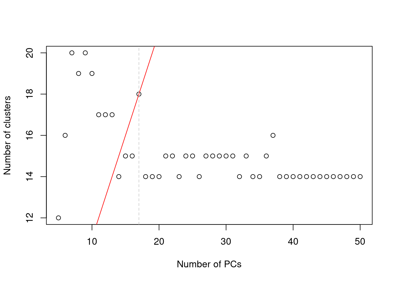
Figure 4.2: Number of clusters detected in the Zeisel brain dataset as a function of the number of PCs. The red unbroken line represents the theoretical upper constraint on the number of clusters, while the grey dashed line is the number of PCs suggested by getClusteredPCs().
We subset the PC matrix by column to retain the first \(d\) PCs
and assign the subsetted matrix back into our SingleCellExperiment object.
Downstream applications that use the "PCA.clust" results in sce.zeisel will subsequently operate on the chosen PCs only.
This strategy is pragmatic as it directly addresses the role of the bias-variance trade-off in downstream analyses, specifically clustering. There is no need to preserve biological signal beyond what is distinguishable in later steps. However, it involves strong assumptions about the nature of the biological differences between subpopulations - and indeed, discrete subpopulations may not even exist in studies of continuous processes like differentiation. It also requires repeated applications of the clustering procedure on increasing number of PCs, which may be computational expensive.
4.2.4 Using random matrix theory
We consider the observed (log-)expression matrix to be the sum of (i) a low-rank matrix containing the true biological signal for each cell and (ii) a random matrix representing the technical noise in the data. Under this interpretation, we can use random matrix theory to guide the choice of the number of PCs based on the properties of the noise matrix.
The Marchenko-Pastur (MP) distribution defines an upper bound on the singular values of a matrix with random i.i.d. entries.
Thus, all PCs associated with larger singular values are likely to contain real biological structure -
or at least, signal beyond that expected by noise - and should be retained (Shekhar et al. 2016).
We can implement this scheme using the chooseMarchenkoPastur() function from the PCAtools package,
given the dimensionality of the matrix used for the PCA (noting that we only used the HVG subset);
the variance explained by each PC (not the percentage);
and the variance of the noise matrix derived from our previous variance decomposition results.
# Generating more PCs for demonstration purposes:
set.seed(10100101)
sce.zeisel2 <- fixedPCA(sce.zeisel, subset.row=top.zeisel, rank=200)

# Actual variance explained is also provided in the attributes:
mp.choice <- chooseMarchenkoPastur(
    .dim=c(length(top.zeisel), ncol(sce.zeisel2)),
    var.explained=attr(reducedDim(sce.zeisel2), "varExplained"),
    noise=median(dec.zeisel[top.zeisel,"tech"]))

mp.choice
## [1] 144
## attr(,"limit")
## [1] 2.336We can then subset the PC coordinate matrix by the first mp.choice columns as previously demonstrated.
It is best to treat this as a guideline only; PCs below the MP limit are not necessarily uninteresting, especially in noisy datasets where the higher noise drives a more aggressive choice of \(d\).
Conversely, many PCs above the limit may not be relevant if they are driven by uninteresting biological processes like transcriptional bursting, cell cycle or metabolic variation.
Morever, the use of the MP distribution is not entirely justified here as the noise distribution differs by abundance for each gene and by sequencing depth for each cell.
In a similar vein, Horn’s parallel analysis is commonly used to pick the number of PCs to retain in factor analysis. This involves randomizing the input matrix, repeating the PCA and creating a scree plot of the PCs of the randomized matrix. The desired number of PCs is then chosen based on the intersection of the randomized scree plot with that of the original matrix (Figure 4.3). Here, the reasoning is that PCs are unlikely to be interesting if they explain less variance that that of the corresponding PC of a random matrix. Note that this differs from the MP approach as we are not using the upper bound of randomized singular values to threshold the original PCs.
set.seed(100010)
horn <- parallelPCA(logcounts(sce.zeisel)[top.zeisel,],
    BSPARAM=BiocSingular::IrlbaParam(), niters=10)
horn$n
## [1] 26plot(horn$original$variance, type="b", log="y", pch=16)
permuted <- horn$permuted
for (i in seq_len(ncol(permuted))) {
points(permuted[,i], col="grey80", pch=16)
lines(permuted[,i], col="grey80", pch=16)
}
abline(v=horn$n, col="red")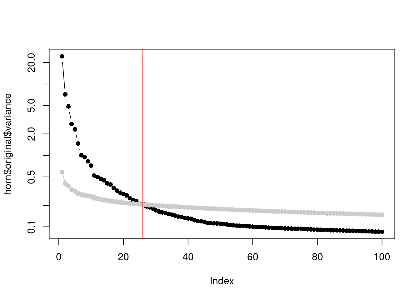
Figure 4.3: Percentage of variance explained by each PC in the original matrix (black) and the PCs in the randomized matrix (grey) across several randomization iterations. The red line marks the chosen number of PCs.
The parallelPCA() function helpfully emits the PC coordinates in horn$original$rotated,
which we can subset by horn$n and add to the reducedDims() of our SingleCellExperiment.
Parallel analysis is reasonably intuitive (as random matrix methods go) and avoids any i.i.d. assumption across genes.
However, its obvious disadvantage is the not-insignificant computational cost of randomizing and repeating the PCA.
One can also debate whether the scree plot of the randomized matrix is even comparable to that of the original,
given that the former includes biological variation and thus cannot be interpreted as purely technical noise.
This manifests in Figure 4.3 as a consistently higher curve for the randomized matrix due to the redistribution of biological variation to the later PCs.
Another approach is based on optimizing the reconstruction error of the low-rank representation (Gavish and Donoho 2014).
Recall that PCA produces both the matrix of per-cell coordinates and a rotation matrix of per-gene loadings,
the product of which recovers the original log-expression matrix.
If we subset these two matrices to the first \(d\) dimensions, the product of the resulting submatrices serves as an approximation of the original matrix.
Under certain conditions, the difference between this approximation and the true low-rank signal (i.e., sans the noise matrix) has a defined mininum at a certain number of dimensions.
This minimum can be defined using the chooseGavishDonoho() function from PCAtools as shown below.
gv.choice <- chooseGavishDonoho(
    .dim=c(length(top.zeisel), ncol(sce.zeisel2)),
    var.explained=attr(reducedDim(sce.zeisel2), "varExplained"),
    noise=median(dec.zeisel[top.zeisel,"tech"]))

gv.choice
## [1] 59
## attr(,"limit")
## [1] 3.121The Gavish-Donoho method is appealing as, unlike the other approaches for choosing \(d\), the concept of the optimum is rigorously defined. By minimizing the reconstruction error, we can most accurately represent the true biological variation in terms of the distances between cells in PC space. However, there remains some room for difference between “optimal” and “useful”; for example, noisy datasets may find themselves with very low \(d\) as including more PCs will only ever increase reconstruction error, regardless of whether they contain relevant biological variation. This approach is also dependent on some strong i.i.d. assumptions about the noise matrix.
4.3 Count-based dimensionality reduction
For count matrices, correspondence analysis (CA) is a natural approach to dimensionality reduction. In this procedure, we compute an expected value for each entry in the matrix based on the per-gene abundance and size factors. Each count is converted into a standardized residual in a manner analogous to the calculation of the statistic in Pearson’s chi-squared tests, i.e., subtraction of the expected value and division by its square root. An SVD is then applied on this matrix of residuals to obtain the necessary low-dimensional coordinates for each cell. To demonstrate, we use the corral package to compute CA factors for the Zeisel dataset.
library(corral)
sce.corral <- corral_sce(sce.zeisel, subset_row=top.zeisel,
   col.w=sizeFactors(sce.zeisel))
dim(reducedDim(sce.corral, "corral"))
## [1] 2816 30The major advantage of CA is that it avoids difficulties with the mean-variance relationship upon transformation (Figure 2.2). If two cells have the same expression profile but differences in their total counts, CA will return the same expected location for both cells; this avoids artifacts observed in PCA on log-transformed counts (Figure 4.4). However, CA is more sensitive to overdispersion in the random noise due to the nature of its standardization. This may cause some problems in some datasets where the CA factors may be driven by a few genes with random expression rather than the underlying biological structure.
# TODO: move to scRNAseq. The rm(env) avoids problems with knitr caching inside
# rebook's use of callr::r() during compilation.
library(BiocFileCache)
bfc <- BiocFileCache(ask=FALSE)
qcdata <- bfcrpath(bfc, "https://github.com/LuyiTian/CellBench_data/blob/master/data/mRNAmix_qc.RData?raw=true")

env <- new.env()
load(qcdata, envir=env)
sce.8qc <- env$sce8_qc
rm(env)

sce.8qc$mix <- factor(sce.8qc$mix)
sce.8qc
## class: SingleCellExperiment
## dim: 15571 296
## metadata(2): scPipe Biomart
## assays(1): counts
## rownames(15571): ENSG00000245025 ENSG00000257433 ... ENSG00000233117
## ENSG00000115687
## rowData names(0):
## colnames(296): L19 A10 ... P8 P9
## colData names(21): unaligned aligned_unmapped ... HCC827_prop
## mRNA_amount
## reducedDimNames(0):
## mainExpName: NULL
## altExpNames(0):# Choosing some HVGs for PCA:
sce.8qc <- logNormCounts(sce.8qc)
dec.8qc <- modelGeneVar(sce.8qc)
hvgs.8qc <- getTopHVGs(dec.8qc, n=1000)
sce.8qc <- fixedPCA(sce.8qc, subset.row=hvgs.8qc)
# By comparison, corral operates on the raw counts:
sce.8qc <- corral_sce(sce.8qc, subset_row=hvgs.8qc, col.w=sizeFactors(sce.8qc))
library(scater)
gridExtra::grid.arrange(
plotPCA(sce.8qc, colour_by="mix") + ggtitle("PCA"),
plotReducedDim(sce.8qc, "corral", colour_by="mix") + ggtitle("corral"),
ncol=2
)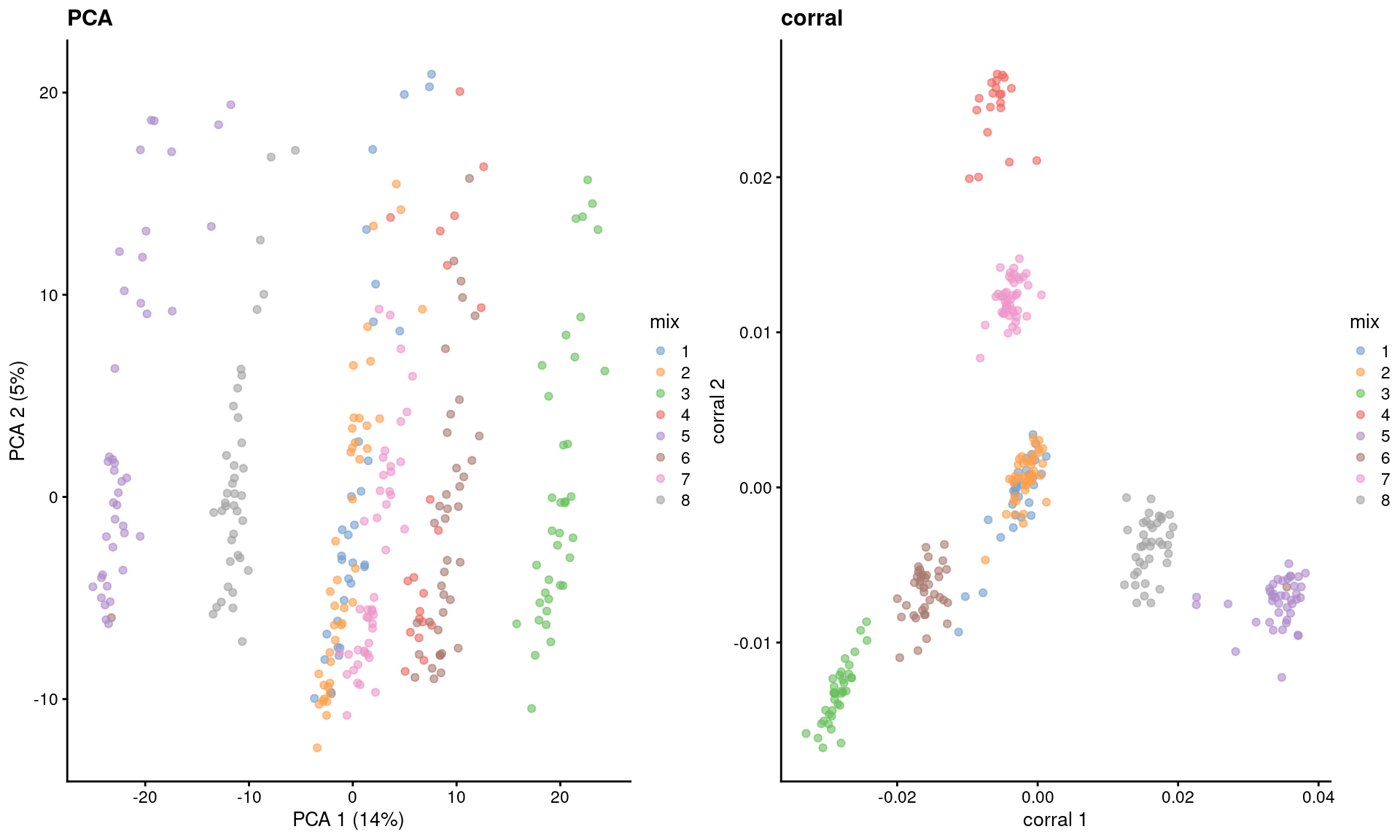
Figure 4.4: Dimensionality reduction results of all pool-and-split libraries in the SORT-seq CellBench data, computed by a PCA on the log-normalized expression values (left) or using the corral package (right). Each point represents a library and is colored by the mixing ratio used to construct it.
4.4 More visualization methods
4.4.1 Fast interpolation-based \(t\)-SNE
Conventional \(t\)-SNE algorithms scale poorly with the number of cells.
Fast interpolation-based \(t\)-SNE (FIt-SNE) (Linderman et al. 2019) is an alternative algorithm that reduces the computational complexity of the calculations from \(N\log N\) to \(\sim 2 p N\).
This is achieved by using interpolation nodes in the high-dimensional space;
the bulk of the calculations are performed on the nodes and the embedding of individual cells around each node is determined by interpolation.
To use this method, we can simply set use_fitsne=TRUE when calling runTSNE() with scater -
this calls the snifter package, which in turn wraps the Python library openTSNE using basilisk
As Figure 4.5 shows, the embeddings produced by this method are qualitatively similar to those produced by other algorithms,
supported by some theoretical results from Linderman et al. (2019) showing that any difference from conventional \(t\)-SNE implementations is low and bounded.
set.seed(9000)
sce.zeisel <- runTSNE(sce.zeisel)
sce.zeisel <- runTSNE(sce.zeisel, use_fitsne = TRUE, name="FIt-SNE")

gridExtra::grid.arrange(
    plotReducedDim(sce.zeisel, "TSNE", colour_by="level1class") + ggtitle("t-SNE"),
    plotReducedDim(sce.zeisel, "FIt-SNE", colour_by="level1class") + ggtitle("FIt-SNE"),
    ncol=2
)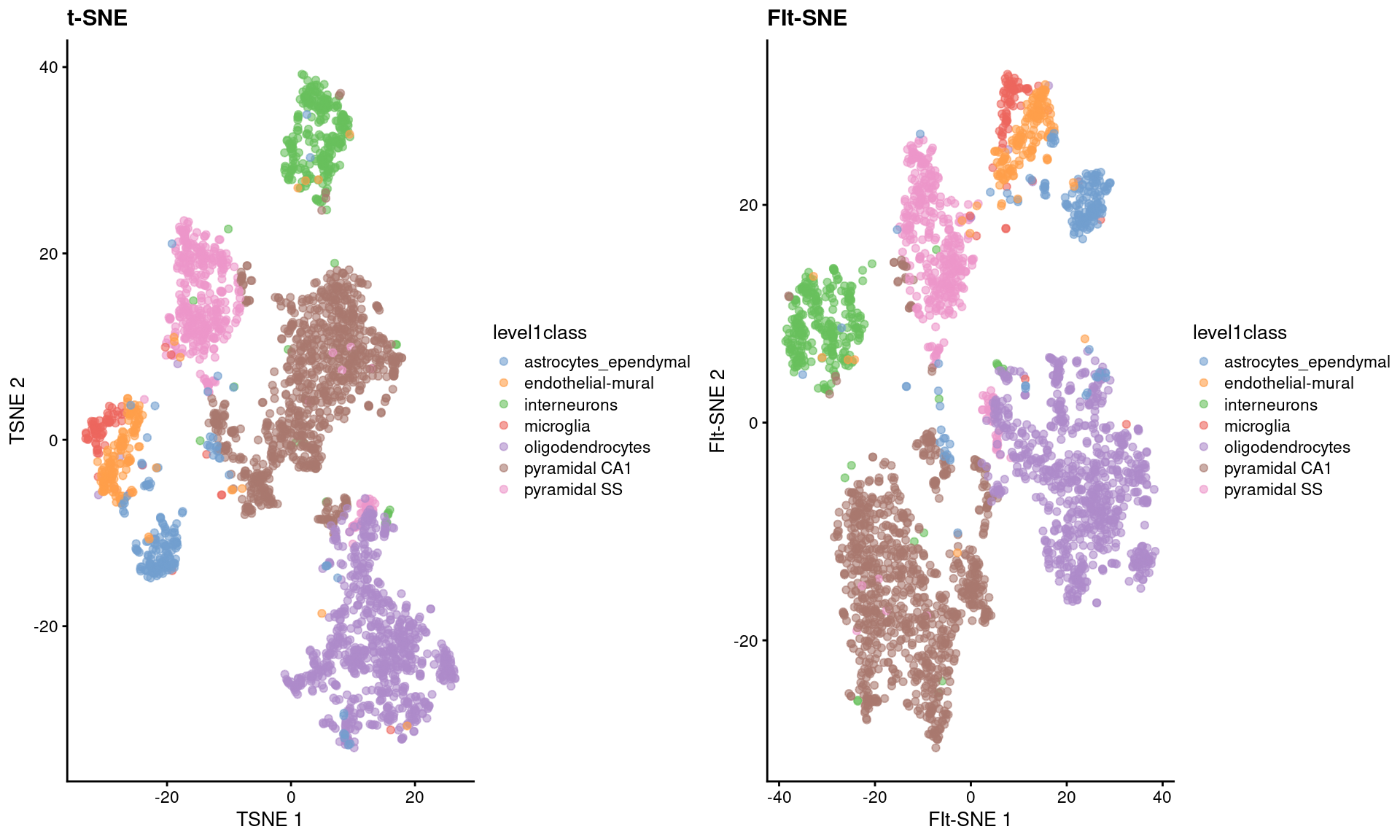
Figure 4.5: FI-tSNE embedding and Barnes-Hut \(t\)-SNE embeddings for the Zeisel brain data.
By using snifter directly, we can also take advantage of openTSNE’s ability to project new points into an existing embedding. In this process, the existing points remain static while new points are inserted based on their affinities with each other and the points in the existing embedding. For example, cells are generally projected near to cells of a similar type in Figure 4.6. This may be useful as an exploratory step when combining datasets, though the projection may not be sensible for cell types that are not present in the existing embedding.
set.seed(1000)
ind_test <- as.logical(rbinom(ncol(sce.zeisel), 1, 0.2))
ind_train <- !ind_test

library(snifter)
olddata <- reducedDim(sce.zeisel[, ind_train], "PCA")
embedding <- fitsne(olddata)
newdata <- reducedDim(sce.zeisel[, ind_test], "PCA")
projected <- project(embedding, new = newdata, old = olddata)

all <- rbind(embedding, projected)
label <- c(sce.zeisel$level1class[ind_train], sce.zeisel$level1class[ind_test])

ggplot() +
    aes(all[, 1], all[, 2], col = factor(label), shape = ind_test) +
    labs(x = "t-SNE 1", y = "t-SNE 2") +
    geom_point(alpha = 0.5) +
    scale_colour_brewer(palette = "Set2", name="level1class") +
    theme_bw() +
    scale_shape_manual(values = c(8, 19), name = "Set", labels = c("Training", "Test"))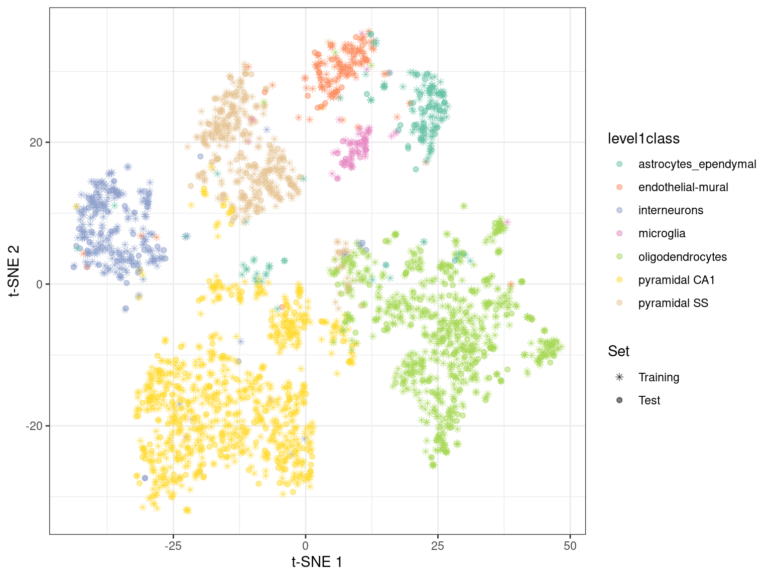
Figure 4.6: \(t\)-SNE embedding created with snifter, using 80% of the cells in the Zeisel brain data. The remaining 20% of the cells were projected into this pre-existing embedding.
4.4.2 Density-preserving \(t\)-SNE and UMAP
One downside of t\(-\)SNE and UMAP is that they preserve the neighbourhood structure of the data while neglecting the local density of the data. This can result in seemingly compact clusters on a t-SNE or UMAP plot that correspond to very heterogeneous groups in the original data. The dens-SNE and densMAP algorithms mitigate this effect by incorporating information about the average distance to the nearest neighbours when creating the embedding (Narayan 2021). We demonstrate below by applying these approaches on the PCs of the Zeisel dataset using the densviz wrapper package.
library(densvis)
dt <- densne(reducedDim(sce.zeisel, "PCA"), dens_frac = 0.4, dens_lambda = 0.2)
reducedDim(sce.zeisel, "dens-SNE") <- dt
dm <- densmap(reducedDim(sce.zeisel, "PCA"), dens_frac = 0.4, dens_lambda = 0.2)
reducedDim(sce.zeisel, "densMAP") <- dm
sce.zeisel <- runUMAP(sce.zeisel) # for comparison
These methods provide more information about transcriptional heterogeneity within clusters (Figure 4.7), with the astrocyte cluster being less compact in the density-preserving versions. This excessive compactness can imply a lower level of within-population heterogeneity.
gridExtra::grid.arrange(
    plotReducedDim(sce.zeisel, "TSNE", colour_by="level1class") + ggtitle("t-SNE"),
    plotReducedDim(sce.zeisel, "dens-SNE", colour_by="level1class") + ggtitle("dens-SNE"),
    plotReducedDim(sce.zeisel, "UMAP", colour_by="level1class") + ggtitle("UMAP"),
    plotReducedDim(sce.zeisel, "densMAP", colour_by="level1class") + ggtitle("densMAP"),
    ncol=2
)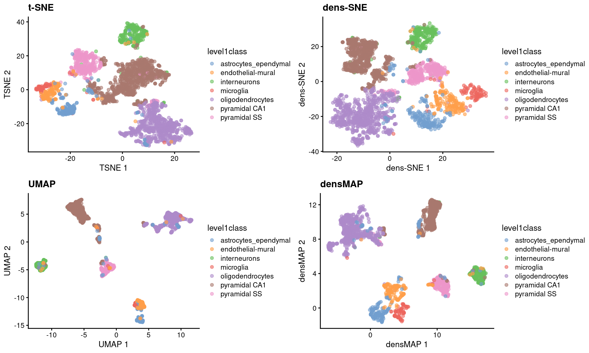
Figure 4.7: \(t\)-SNE, UMAP, dens-SNE and densMAP embeddings for the Zeisel brain data.
Session Info
R version 4.2.2 (2022-10-31)
Platform: x86_64-pc-linux-gnu (64-bit)
Running under: Ubuntu 20.04.5 LTS

Matrix products: default
BLAS:   /home/biocbuild/bbs-3.16-bioc/R/lib/libRblas.so
LAPACK: /home/biocbuild/bbs-3.16-bioc/R/lib/libRlapack.so

locale:
 [1] LC_CTYPE=en_US.UTF-8       LC_NUMERIC=C
 [3] LC_TIME=en_GB              LC_COLLATE=C
 [5] LC_MONETARY=en_US.UTF-8    LC_MESSAGES=en_US.UTF-8
 [7] LC_PAPER=en_US.UTF-8       LC_NAME=C
 [9] LC_ADDRESS=C               LC_TELEPHONE=C
[11] LC_MEASUREMENT=en_US.UTF-8 LC_IDENTIFICATION=C

attached base packages:
[1] stats4    stats     graphics  grDevices utils     datasets  methods
[8] base

other attached packages:
 [1] densvis_1.8.3               snifter_1.8.0
 [3] scater_1.26.1               BiocFileCache_2.6.0
 [5] dbplyr_2.3.0                corral_1.8.0
 [7] PCAtools_2.10.0             ggrepel_0.9.2
 [9] ggplot2_3.4.0               scran_1.26.2
[11] scuttle_1.8.4               SingleCellExperiment_1.20.0
[13] SummarizedExperiment_1.28.0 Biobase_2.58.0
[15] GenomicRanges_1.50.2        GenomeInfoDb_1.34.8
[17] IRanges_2.32.0              S4Vectors_0.36.1
[19] BiocGenerics_0.44.0         MatrixGenerics_1.10.0
[21] matrixStats_0.63.0          BiocStyle_2.26.0
[23] rebook_1.8.0

loaded via a namespace (and not attached):
  [1] plyr_1.8.8                  igraph_1.3.5
  [3] BiocParallel_1.32.5         digest_0.6.31
  [5] htmltools_0.5.4             viridis_0.6.2
  [7] fansi_1.0.4                 magrittr_2.0.3
  [9] RMTstat_0.3.1               memoise_2.0.1
 [11] ScaledMatrix_1.6.0          cluster_2.1.4
 [13] limma_3.54.1                colorspace_2.1-0
 [15] blob_1.2.3                  rappdirs_0.3.3
 [17] xfun_0.36                   dplyr_1.1.0
 [19] RCurl_1.98-1.10             jsonlite_1.8.4
 [21] graph_1.76.0                glue_1.6.2
 [23] pals_1.7                    gtable_0.3.1
 [25] zlibbioc_1.44.0             XVector_0.38.0
 [27] DelayedArray_0.24.0         BiocSingular_1.14.0
 [29] maps_3.4.1                  scales_1.2.1
 [31] DBI_1.1.3                   edgeR_3.40.2
 [33] ggthemes_4.2.4              Rcpp_1.0.10
 [35] viridisLite_0.4.1           reticulate_1.28
 [37] dqrng_0.3.0                 bit_4.0.5
 [39] rsvd_1.0.5                  mapproj_1.2.11
 [41] metapod_1.6.0               httr_1.4.4
 [43] FNN_1.1.3.1                 dir.expiry_1.6.0
 [45] RColorBrewer_1.1-3          pkgconfig_2.0.3
 [47] XML_3.99-0.13               farver_2.1.1
 [49] CodeDepends_0.6.5           sass_0.4.5
 [51] uwot_0.1.14                 locfit_1.5-9.7
 [53] utf8_1.2.3                  here_1.0.1
 [55] tidyselect_1.2.0            labeling_0.4.2
 [57] rlang_1.0.6                 reshape2_1.4.4
 [59] munsell_0.5.0               tools_4.2.2
 [61] cachem_1.0.6                cli_3.6.0
 [63] generics_0.1.3              RSQLite_2.2.20
 [65] evaluate_0.20               stringr_1.5.0
 [67] fastmap_1.1.0               yaml_2.3.7
 [69] transport_0.13-0            knitr_1.42
 [71] bit64_4.0.5                 purrr_1.0.1
 [73] sparseMatrixStats_1.10.0    compiler_4.2.2
 [75] beeswarm_0.4.0              filelock_1.0.2
 [77] curl_5.0.0                  png_0.1-8
 [79] tibble_3.1.8                statmod_1.5.0
 [81] bslib_0.4.2                 stringi_1.7.12
 [83] highr_0.10                  basilisk.utils_1.10.0
 [85] lattice_0.20-45             bluster_1.8.0
 [87] Matrix_1.5-3                vctrs_0.5.2
 [89] pillar_1.8.1                lifecycle_1.0.3
 [91] BiocManager_1.30.19         jquerylib_0.1.4
 [93] BiocNeighbors_1.16.0        data.table_1.14.6
 [95] cowplot_1.1.1               bitops_1.0-7
 [97] irlba_2.3.5.1               R6_2.5.1
 [99] bookdown_0.32               gridExtra_2.3
[101] vipor_0.4.5                 codetools_0.2-18
[103] dichromat_2.0-0.1           assertthat_0.2.1
[105] rprojroot_2.0.3             withr_2.5.0
[107] GenomeInfoDbData_1.2.9      parallel_4.2.2
[109] MultiAssayExperiment_1.24.0 grid_4.2.2
[111] beachmat_2.14.0             basilisk_1.10.2
[113] rmarkdown_2.20              DelayedMatrixStats_1.20.0
[115] Rtsne_0.16                  ggbeeswarm_0.7.1
References
Gavish, M., and D. L. Donoho. 2014. “The Optimal Hard Threshold for Singular Values Is \(4/\sqrt {3}\).” IEEE Transactions on Information Theory 60 (8): 5040–53.
Linderman, George C., Manas Rachh, Jeremy G. Hoskins, Stefan Steinerberger, and Yuval Kluger. 2019. “Fast Interpolation-Based T-SNE for Improved Visualization of Single-Cell RNA-Seq Data.” Nature Methods 16 (3): 243–45. https://doi.org/10.1038/s41592-018-0308-4.
Narayan, Ashwin. 2021. “Assessing Single-Cell Transcriptomic Variability Through Density-Preserving Data Visualization.” Nature Biotechnology, 19. https://doi.org/10.1038/s41587-020-00801-7.
Shekhar, K., S. W. Lapan, I. E. Whitney, N. M. Tran, E. Z. Macosko, M. Kowalczyk, X. Adiconis, et al. 2016. “Comprehensive Classification of Retinal Bipolar Neurons by Single-Cell Transcriptomics.” Cell 166 (5): 1308–23.
Zeisel, A., A. B. Munoz-Manchado, S. Codeluppi, P. Lonnerberg, G. La Manno, A. Jureus, S. Marques, et al. 2015. “Brain structure. Cell types in the mouse cortex and hippocampus revealed by single-cell RNA-seq.” Science 347 (6226): 1138–42.