Chapter 2 Counting reads into windows
2.1 Background
The key step in the DB analysis is the manner in which reads are counted. The most obvious strategy is to count reads into pre-defined regions of interest, like promoters or gene bodies (???). This is simple but will not capture changes outside of those regions. In contrast, de novo analyses do not depend on pre-specified regions, instead using empirically defined peaks or sliding windows for read counting. Peak-based methods are implemented in the DiffBind and DBChIP software packages (Ross-Innes et al. 2012; ???), which count reads into peak intervals that have been identified with software like MACS (???). This requires some care to maintain statistical rigour as peaks are called with the same data used to test for DB.
Alternatively, window-based approaches count reads into sliding windows across the genome. This is a more direct strategy that avoids problems with data re-use and can provide increased DB detection power (???). In csaw, we define a window as a fixed-width genomic interval and we count the number of fragments overlapping that window in each library. For single-end data, each fragment is imputed by directional extension of the read to the average fragment length (Figure 2.1), while for paired-end data, the fragment is defined from the interval spanned by the paired reads. This is repeated after sliding the window along the genome to a new position. A count is then obtained for each window in each library, thus quantifying protein binding intensity across the genome.
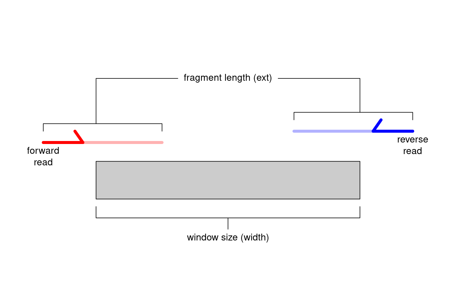
Figure 2.1: Schematic of the read extension process for single-end data. Reads are extended to the average fragment length (ext) and the number of overlapping extended reads is counted for each window of size width.
For single-end data, we estimate the average fragment length from a cross-correlation plot (see Section 2.4) for use as ext.
Alternatively, the length can be estimated from diagnostics during ChIP or library preparation, e.g., post-fragmentation gel electrophoresis images.
Typical values range from 100 to 300 bp, depending on the efficiency of sonication and the use of size selection steps in library preparation.
We interpret the window size (width) as the width of the binding site for the target protein, i.e., its physical “footprint” on the genome.
This is user-specified and has important implications for the power and resolution of a DB analysis, which are discussed in Section 2.5.
For TF analyses with small windows, the choice of spacing interval will also be affected by the choice of window size – see Section 3.2 for more details.
2.2 Obtaining window-level counts
To demonstrate, we will use some publicly available data from the chipseqDBData package. The dataset below focuses on changes in the binding profile of the NF-YA transcription factor between embryonic stem cells and terminal neurons (Tiwari et al. 2012).
## DataFrame with 5 rows and 3 columns
##          Name   Description      Path
##   <character>   <character>    <List>
## 1   SRR074398 NF-YA ESC (1) <BamFile>
## 2   SRR074399 NF-YA ESC (2) <BamFile>
## 3   SRR074417  NF-YA TN (1) <BamFile>
## 4   SRR074418  NF-YA TN (2) <BamFile>
## 5 SRR074401 Input <BamFile>## List of length 4The windowCounts() function uses a sliding window approach to count fragments for a set of BAM files,
supplied as either a character vector or as a list of BamFile objects (from the Rsamtools package).
We assume that the BAM files are sorted by position and have been indexed - for character inputs, the index files are assumed to have the same prefixes as the BAM files.
It’s worth pointing out that a common mistake is to replace or update the BAM file without updating the index, which will cause csaw some grief.
library(csaw)
frag.len <- 110
win.width <- 10
param <- readParam(minq=20)
data <- windowCounts(bam.files, ext=frag.len, width=win.width, param=param)
The function returns a RangedSummarizedExperiment object where the matrix of counts is stored as the first assay.
Each row corresponds to a genomic window while each column corresponds to a library.
The coordinates of each window are stored in the rowRanges.
The total number of reads in each library (also referred to as the library size) is stored as totals in the colData.
##      [,1] [,2] [,3] [,4]
## [1,]    2    3    3    4
## [2,]    3    6    3    4
## [3,]    5    5    0    0
## [4,]    4    7    0    0
## [5,]    5    9    0    0
## [6,] 3 9 0 0## GRanges object with 6 ranges and 0 metadata columns:
## seqnames ranges strand
## <Rle> <IRanges> <Rle>
## [1] chr1 3003701-3003710 *
## [2] chr1 3003751-3003760 *
## [3] chr1 3003801-3003810 *
## [4] chr1 3003951-3003960 *
## [5] chr1 3004001-3004010 *
## [6] chr1 3004051-3004060 *
## -------
## seqinfo: 66 sequences from an unspecified genome## [1] 18363361 21752369 25095004 24104691The above windowCounts() call involved a few arguments, so we will spend the rest of this chapter explaining these in more detail.
2.3 Filtering out low-quality reads
Read extraction from the BAM files is controlled with the param argument in windowCounts().
This takes a readParam object that specifies a number of extraction parameters.
The idea is to define the readParam object once in the entire analysis pipeline, which is then reused for all relevant functions.
This ensures that read loading is consistent throughout the analysis.
(A good measure of synchronisation between windowCounts() calls is to check that the values of totals are identical between calls,
which indicates that the same reads are being extracted from the BAM files in each call.)
##     Extracting reads in single-end mode
##     Duplicate removal is turned off
##     Minimum allowed mapping score is 20
##     Reads are extracted from both strands
##     No restrictions are placed on read extraction
##     No regions are specified to discard reads
In the example above, reads are filtered out based on the minimum mapping score with the minq argument.
Low mapping scores are indicative of incorrectly and/or non-uniquely aligned sequences.
Removal of these reads is highly recommended as it will ensure that only the reliable alignments are supplied to csaw.
The exact value of the threshold depends on the range of scores provided by the aligner.
The subread aligner (Liao, Smyth, and Shi 2013) was used to align the reads in this dataset, so a value of 20 might be appropriate.
Reads mapping to the same genomic position can be marked as putative PCR duplicates using software like the MarkDuplicates program from the Picard suite.
Marked reads in the BAM file can be ignored during counting by setting dedup=TRUE in the readParam object.
This reduces the variability caused by inconsistent amplification between replicates, and avoid spurious duplicate-driven DB between groups.
An example of counting with duplicate removal is shown below, where fewer reads are used from each library relative to data\$totals.
dedup.param <- readParam(minq=20, dedup=TRUE)
demo <- windowCounts(bam.files, ext=frag.len, width=win.width,
    param=dedup.param)
demo$totals
## [1] 14799759 14773466 17424949 20386739That said, duplicate removal is generally not recommended for routine DB analyses. This is because it caps the number of reads at each position, reducing DB detection power in high-abundance regions. Spurious differences may also be introduced when the same upper bound is applied to libraries of varying size. However, it may be unavoidable in some cases, e.g., involving libraries generated from low quantities of DNA. Duplicate removal is also acceptable for paired-end data, as exact overlaps for both paired reads are required to define duplicates. This greatly reduces the probability of incorrectly discarding read pairs from non-duplicate DNA fragments (assuming that a pair-aware method was used during duplicate marking).
2.4 Estimating the fragment length
Cross-correlation plots are generated directly from BAM files using the correlateReads() function.
This provides a measure of the immunoprecipitation (IP) efficiency of a ChIP-seq experiment (Kharchenko, Tolstorukov, and Park 2008).
Efficient IP should yield a smooth peak at a delay distance corresponding to the average fragment length.
This reflects the strand-dependent bimodality of reads around narrow regions of enrichment, e.g., TF binding sites.
max.delay <- 500
dedup.on <- initialize(param, dedup=TRUE) # just flips 'dedup=TRUE' in the existing 'param'.
x <- correlateReads(bam.files, max.delay, param=dedup.on)
plot(0:max.delay, x, type="l", ylab="CCF", xlab="Delay (bp)")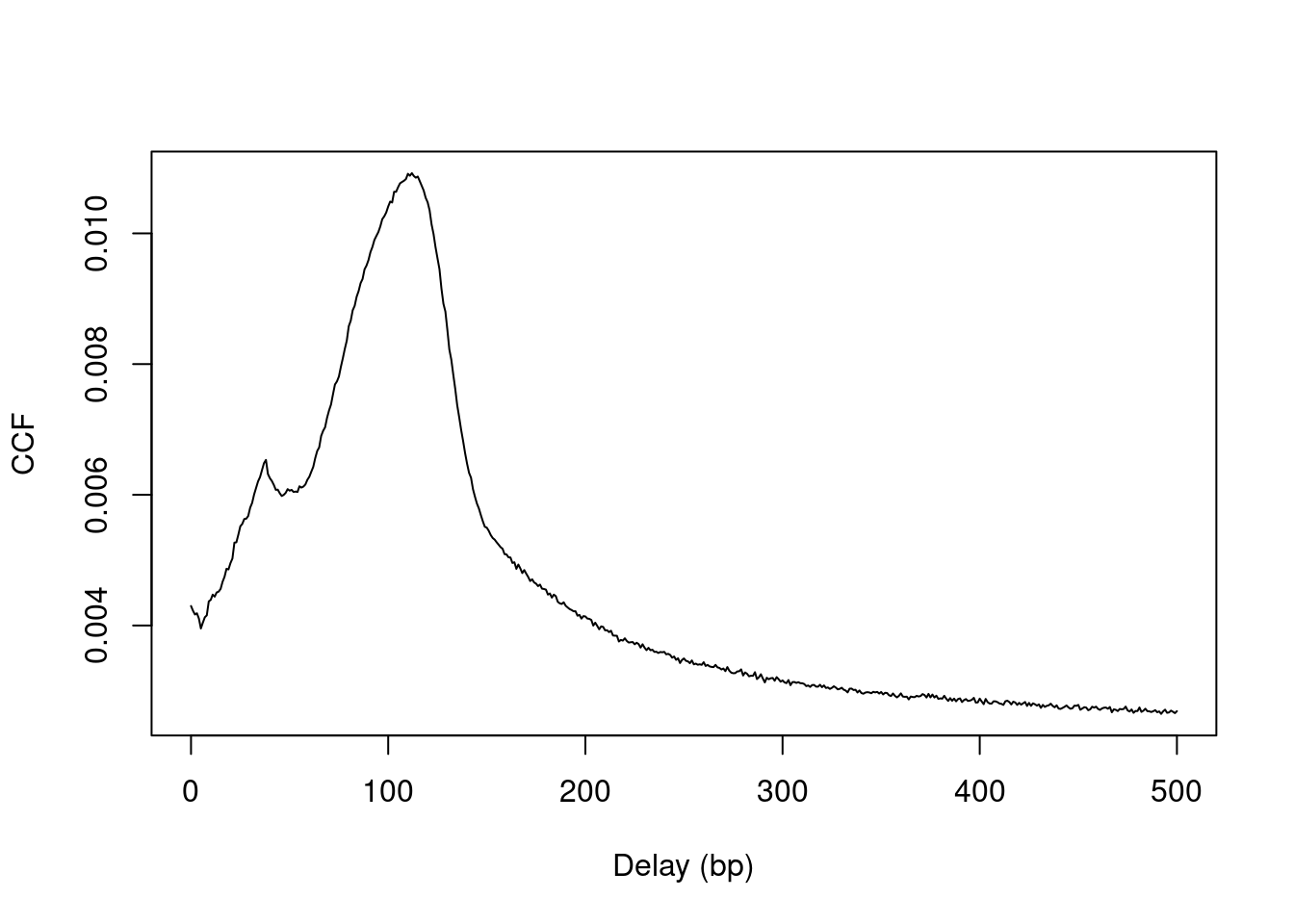
Figure 2.2: Cross-correlation plot of the NF-YA dataset.
The location of the peak is used as an estimate of the fragment length for read extension in windowCounts().
An estimate of ~110 bp is obtained from the plot above.
We can do this more precisely with the maximizeCcf() function, which returns a similar value.
## [1] 112A sharp spike may also be observed in the plot at a distance corresponding to the read length.
This is thought to be an artifact, caused by the preference of aligners towards uniquely mapped reads.
Duplicate removal is typically required here (i.e., set dedup=TRUE in readParam()) to reduce the size of this spike.
Otherwise, the fragment length peak will not be visible as a separate entity.
The size of the smooth peak can also be compared to the height of the spike to assess the signal-to-noise ratio of the data (Landt et al. 2012).
Poor IP efficiency will result in a smaller or absent peak as bimodality is less pronounced.
Cross-correlation plots can also be used for fragment length estimation of narrow histone marks such as histone acetylation and H3K4 methylation (Figure 2.3). However, they are less effective for regions of diffuse enrichment where bimodality is not obvious (e.g., H3K27 trimethylation).
n <- 1000

# Using more data sets from 'chipseqDBData'.
acdata <- H3K9acData()
h3k9ac <- correlateReads(acdata$Path[1], n, param=dedup.on)

k27data <- H3K27me3Data()
h3k27me3 <- correlateReads(k27data$Path[1], n, param=dedup.on)

k4data <- H3K4me3Data()
h3k4me3 <- correlateReads(k4data$Path[1], n, param=dedup.on)

plot(0:n, h3k9ac, col="blue", ylim=c(0, 0.1), xlim=c(0, 1000),
     xlab="Delay (bp)", ylab="CCF", pch=16, type="l", lwd=2)
lines(0:n, h3k27me3, col="red", pch=16, lwd=2)
lines(0:n, h3k4me3, col="forestgreen", pch=16, lwd=2)
legend("topright", col=c("blue", "red", "forestgreen"),
       c("H3K9ac", "H3K27me3", "H3K4me3"), pch=16)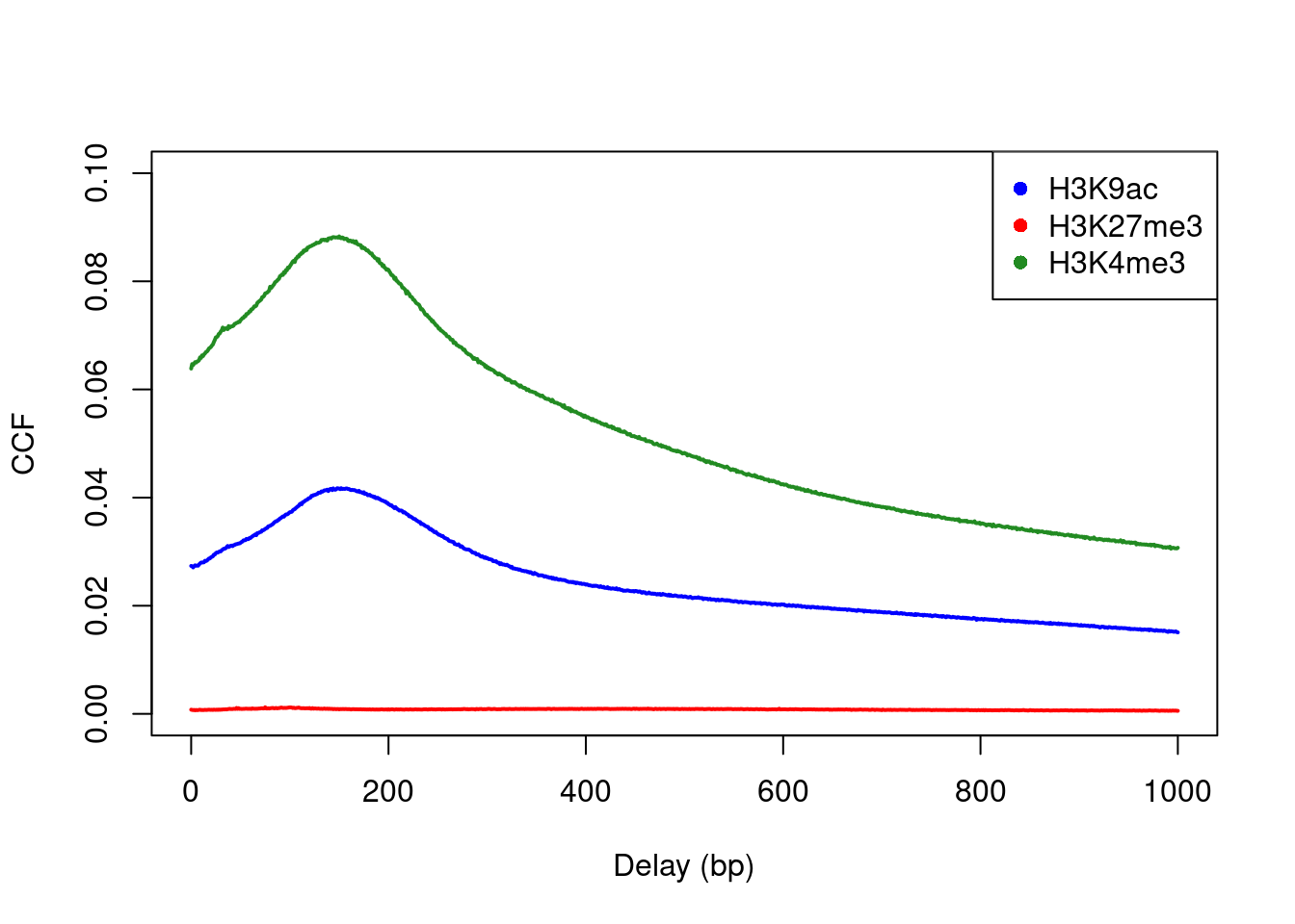
Figure 2.3: Cross-correlation plots for a variety of histone mark datasets.
In general, use of different extension lengths is unnecessary in well-controlled datasets.
Difference in lengths between libraries are usually smaller than 50 bp.
This is less than the inherent variability in fragment lengths within each library (see the histogram for the paired-end data in Section~).
The effect on the coverage profile of within-library variability in lengths will likely mask the effect of small between-library differences in the average lengths.
Thus, an ext list should only be specified for datasets that exhibit large differences in the average fragment sizes between libraries.
2.5 Choosing a window size
We interpret the window size as the width of the binding ``footprint’’ for the target protein, where the protein residues directly contact the DNA. TF analyses typically use a small window size, e.g., 10 - 20 bp, which maximizes spatial resolution for optimal detection of narrow regions of enrichment. For histone marks, widths of at least 150 bp are recommended (Humburg et al. 2011). This corresponds to the length of DNA wrapped up in each nucleosome, which is the smallest relevant unit for histone mark enrichment. We consider diffuse marks as chains of adjacent histones, for which the combined footprint may be very large (e.g., 1-10 kbp).
The choice of window size controls the compromise between spatial resolution and count size. Larger windows will yield larger read counts that can provide more power for DB detection. However, spatial resolution is also lost for large windows whereby adjacent features can no longer be distinguished. Reads from a DB site may be counted alongside reads from a non-DB site (e.g., non-specific background) or even those from an adjacent site that is DB in the opposite direction. This will result in the loss of DB detection power.
We might expect to be able to infer the optimal window size from the data, e.g., based on the width of the enriched regions. However, in practice, a clear-cut choice of distance/window size is rarely found in real datasets. For many non-TF targets, the widths of the enriched regions can be highly variable, suggesting that no single window size is optimal. Indeed, even if all enriched regions were of constant width, the width of the DB events occurring those regions may be variable. This is especially true of diffuse marks where the compromise between resolution and power is more arbitrary.
We suggest performing an initial DB analysis with small windows to maintain spatial resolution. The widths of the final merged regions (see Section~) can provide an indication of the appropriate window size. Alternatively, the analysis can be repeated with a series of larger windows, and the results combined (see Section~). This examines a spread of resolutions for more comprehensive detection of DB regions.
Session information
R version 4.2.1 (2022-06-23)
Platform: x86_64-pc-linux-gnu (64-bit)
Running under: Ubuntu 20.04.4 LTS

Matrix products: default
BLAS:   /home/biocbuild/bbs-3.15-bioc/R/lib/libRblas.so
LAPACK: /home/biocbuild/bbs-3.15-bioc/R/lib/libRlapack.so

locale:
 [1] LC_CTYPE=en_US.UTF-8       LC_NUMERIC=C
 [3] LC_TIME=en_GB              LC_COLLATE=C
 [5] LC_MONETARY=en_US.UTF-8    LC_MESSAGES=en_US.UTF-8
 [7] LC_PAPER=en_US.UTF-8       LC_NAME=C
 [9] LC_ADDRESS=C               LC_TELEPHONE=C
[11] LC_MEASUREMENT=en_US.UTF-8 LC_IDENTIFICATION=C

attached base packages:
[1] stats4    stats     graphics  grDevices utils     datasets  methods
[8] base

other attached packages:
 [1] csaw_1.30.1                 SummarizedExperiment_1.26.1
 [3] Biobase_2.56.0              MatrixGenerics_1.8.1
 [5] matrixStats_0.62.0          GenomicRanges_1.48.0
 [7] GenomeInfoDb_1.32.3         IRanges_2.30.1
 [9] S4Vectors_0.34.0            BiocGenerics_0.42.0
[11] chipseqDBData_1.12.0        BiocStyle_2.24.0
[13] rebook_1.6.0

loaded via a namespace (and not attached):
 [1] bitops_1.0-7                  bit64_4.0.5
 [3] filelock_1.0.2                httr_1.4.4
 [5] tools_4.2.1                   bslib_0.4.0
 [7] utf8_1.2.2                    R6_2.5.1
 [9] DBI_1.1.3                     tidyselect_1.1.2
[11] bit_4.0.4                     curl_4.3.2
[13] compiler_4.2.1                graph_1.74.0
[15] cli_3.3.0                     DelayedArray_0.22.0
[17] bookdown_0.28                 sass_0.4.2
[19] rappdirs_0.3.3                stringr_1.4.1
[21] digest_0.6.29                 Rsamtools_2.12.0
[23] rmarkdown_2.16                XVector_0.36.0
[25] pkgconfig_2.0.3               htmltools_0.5.3
[27] limma_3.52.2                  dbplyr_2.2.1
[29] fastmap_1.1.0                 highr_0.9
[31] rlang_1.0.4                   RSQLite_2.2.16
[33] shiny_1.7.2                   jquerylib_0.1.4
[35] generics_0.1.3                jsonlite_1.8.0
[37] BiocParallel_1.30.3           dplyr_1.0.9
[39] RCurl_1.98-1.8                magrittr_2.0.3
[41] GenomeInfoDbData_1.2.8        Matrix_1.4-1
[43] Rcpp_1.0.9                    fansi_1.0.3
[45] lifecycle_1.0.1               edgeR_3.38.4
[47] stringi_1.7.8                 yaml_2.3.5
[49] zlibbioc_1.42.0               BiocFileCache_2.4.0
[51] AnnotationHub_3.4.0           grid_4.2.1
[53] blob_1.2.3                    parallel_4.2.1
[55] promises_1.2.0.1              ExperimentHub_2.4.0
[57] crayon_1.5.1                  lattice_0.20-45
[59] dir.expiry_1.4.0              Biostrings_2.64.1
[61] KEGGREST_1.36.3               locfit_1.5-9.6
[63] CodeDepends_0.6.5             metapod_1.4.0
[65] knitr_1.40                    pillar_1.8.1
[67] codetools_0.2-18              XML_3.99-0.10
[69] glue_1.6.2                    BiocVersion_3.15.2
[71] evaluate_0.16                 BiocManager_1.30.18
[73] png_0.1-7                     vctrs_0.4.1
[75] httpuv_1.6.5                  purrr_0.3.4
[77] assertthat_0.2.1              cachem_1.0.6
[79] xfun_0.32                     mime_0.12
[81] xtable_1.8-4                  later_1.3.0
[83] tibble_3.1.8                  AnnotationDbi_1.58.0
[85] memoise_2.0.1                 ellipsis_0.3.2
[87] interactiveDisplayBase_1.34.0
Bibliography
Humburg, P., C. A. Helliwell, D. Bulger, and G. Stone. 2011. “ChIPseqR: analysis of ChIP-seq experiments.” BMC Bioinformatics 12: 39.
Kharchenko, P. V., M. Y. Tolstorukov, and P. J. Park. 2008. “Design and analysis of ChIP-seq experiments for DNA-binding proteins.” Nat. Biotechnol. 26 (12): 1351–9.
Landt, S. G., G. K. Marinov, A. Kundaje, P. Kheradpour, F. Pauli, S. Batzoglou, B. E. Bernstein, et al. 2012. “ChIP-seq guidelines and practices of the ENCODE and modENCODE consortia.” Genome Res. 22 (9): 1813–31.
Liao, Y., G. K. Smyth, and W. Shi. 2013. “The Subread aligner: fast, accurate and scalable read mapping by seed-and-vote.” Nucleic Acids Res. 41 (10): e108.
Ross-Innes, C. S., R. Stark, A. E. Teschendorff, K. A. Holmes, H. R. Ali, M. J. Dunning, G. D. Brown, et al. 2012. “Differential oestrogen receptor binding is associated with clinical outcome in breast cancer.” Nature 481 (7381): 389–93.
Tiwari, V. K., M. B. Stadler, C. Wirbelauer, R. Paro, D. Schubeler, and C. Beisel. 2012. “A chromatin-modifying function of JNK during stem cell differentiation.” Nat. Genet. 44 (1): 94–100.