Chapter 4 The SingleCellExperiment class
4.1 Overview
One of the main strengths of the Bioconductor project lies in the use of a common data infrastructure that powers interoperability across packages.
Users should be able to analyze their data using functions from different Bioconductor packages without the need to convert between formats.
To this end, the SingleCellExperiment class (from the SingleCellExperiment package) serves as the common currency for data exchange across 70+ single-cell-related Bioconductor packages.
This class implements a data structure that stores all aspects of our single-cell data - gene-by-cell expression data, per-cell metadata and per-gene annotation (Figure 4.1) - and manipulate them in a synchronized manner.
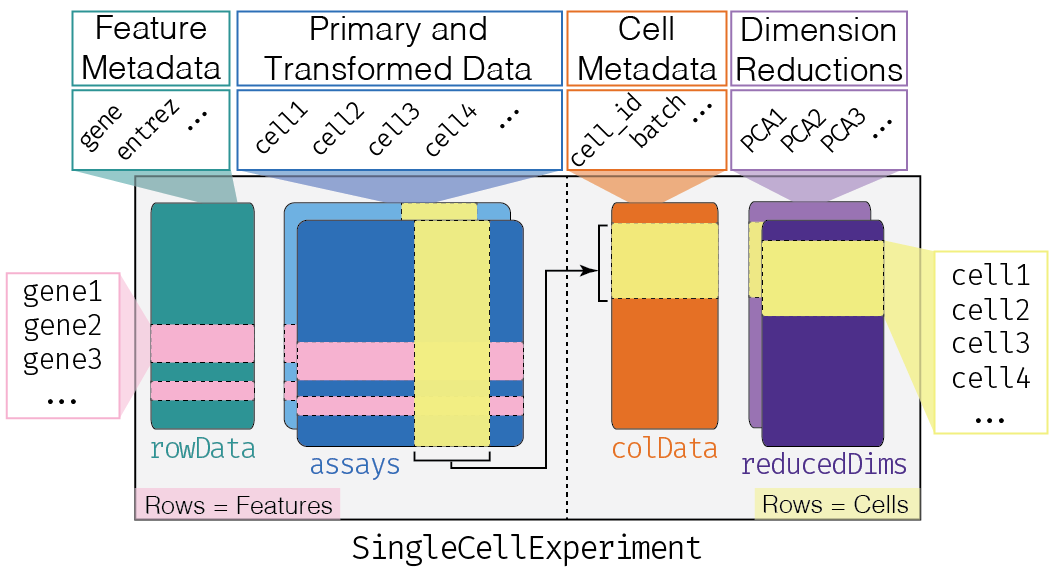
Figure 4.1: Overview of the structure of the SingleCellExperiment class. Each row of the assays corresponds to a row of the rowData (pink shading), while each column of the assays corresponds to a column of the colData and reducedDims (yellow shading).
Each piece of (meta)data in the SingleCellExperiment is represented by a separate “slot”.
(This terminology comes from the S4 class system, but that’s not important right now.)
If we imagine the SingleCellExperiment object to be a cargo ship, the slots can be thought of as individual cargo boxes with different contents, e.g., certain slots expect numeric matrices whereas others may expect data frames.
In the rest of this chapter, we will discuss the available slots, their expected formats, and how we can interact with them.
More experienced readers may note the similarity with the SummarizedExperiment class, and if you are such a reader, you may wish to jump directly to the end of this chapter for the single-cell-specific aspects of this class.
4.2 Installing required packages
The SingleCellExperiment package is automatically installed when using any package that depends on the SingleCellExperiment class, but it can also be explicitly installed:
We then load the SingleCellExperiment package into our R session.
This avoids the need to prefix our function calls with ::, especially for packages that are heavily used throughout a workflow.
For the demonstrations in this chapter, we will use some functions from a variety of other packages, installed as shown below.
These functions will be accessed through the <package>::<function> convention as needed.
4.3 Storing primary experimental data
4.3.1 Filling the assays slot
To construct a rudimentary SingleCellExperiment object, we only need to fill the assays slot.
This contains primary data such as a matrix of sequencing counts where rows correspond to features (genes) and columns correspond to samples (cells) (Figure 4.1, blue box).
To demonstrate, we will use a small scRNA-seq count matrix downloaded from the ArrayExpress servers (Lun et al. 2017):
mat <- read.delim(file.path(tempdir(), "counts_Calero_20160113.tsv"),
    header=TRUE, row.names=1, check.names=FALSE)

# Only considering endogenous genes for now.
spike.mat <- mat[grepl("^ERCC-", rownames(mat)),]
mat <- mat[grepl("^ENSMUSG", rownames(mat)),]

# Splitting off the gene length column.
gene.length <- mat[,1]
mat <- as.matrix(mat[,-1])

dim(mat)
## [1] 46603 96From this, we can now construct our first SingleCellExperiment object using the SingleCellExperiment() function.
Note that we provide our data as a named list where each entry of the list is a matrix - in this case, named "counts".
To inspect the object, we can simply type sce into the console to see some pertinent information.
This will print an overview of the various slots available to us, which may or may not have any data.
## class: SingleCellExperiment
## dim: 46603 96
## metadata(0):
## assays(1): counts
## rownames(46603): ENSMUSG00000102693 ENSMUSG00000064842 ...
##   ENSMUSG00000096730 ENSMUSG00000095742
## rowData names(0):
## colnames(96): SLX-9555.N701_S502.C89V9ANXX.s_1.r_1
##   SLX-9555.N701_S503.C89V9ANXX.s_1.r_1 ...
##   SLX-9555.N712_S508.C89V9ANXX.s_1.r_1
##   SLX-9555.N712_S517.C89V9ANXX.s_1.r_1
## colData names(0):
## reducedDimNames(0):
## mainExpName: NULL
## altExpNames(0):
To access the count data we just supplied, we can do any one of the following:
assay(sce, "counts")- this is the most general method, where we can supply the name of the assay as the second argument.counts(sce)- this is a short-cut for the above, but only works for assays with the special name"counts".
NOTE: For exported S4 classes, it is rarely a good idea to directly access the slots with the @ oeprator.
This is considered bad practice as the class developers are free to alter the internal structure of the class, at which point any code using @ may no longer work.
Rather, it is best to use the provided getter functions like assay() and counts() to extract data from the object.
Similarly, setting slots should be done via the provided setter functions, which are discussed in the next section.
4.3.2 Adding more assays
One of the strengths of the assays slot is that it can hold multiple representations of the primary data.
This is particularly useful for storing the raw count matrix as well as a normalized version of the data.
For example, the logNormCounts() function from scuttle will compute a log-transformed normalized expression matrix and store it as another assay.
## class: SingleCellExperiment
## dim: 46603 96
## metadata(0):
## assays(2): counts logcounts
## rownames(46603): ENSMUSG00000102693 ENSMUSG00000064842 ...
##   ENSMUSG00000096730 ENSMUSG00000095742
## rowData names(0):
## colnames(96): SLX-9555.N701_S502.C89V9ANXX.s_1.r_1
##   SLX-9555.N701_S503.C89V9ANXX.s_1.r_1 ...
##   SLX-9555.N712_S508.C89V9ANXX.s_1.r_1
##   SLX-9555.N712_S517.C89V9ANXX.s_1.r_1
## colData names(1): sizeFactor
## reducedDimNames(0):
## mainExpName: NULL
## altExpNames(0):
We overwrite our previous sce by reassigning the result of logNormCounts() back to sce.
This is possible because these particular functions return a SingleCellExperiment object that contains the results in addition to original data.
Indeed, viewing the object again, we see that this function added a new assay entry "logcounts".
## class: SingleCellExperiment
## dim: 46603 96
## metadata(0):
## assays(2): counts logcounts
## rownames(46603): ENSMUSG00000102693 ENSMUSG00000064842 ...
##   ENSMUSG00000096730 ENSMUSG00000095742
## rowData names(0):
## colnames(96): SLX-9555.N701_S502.C89V9ANXX.s_1.r_1
##   SLX-9555.N701_S503.C89V9ANXX.s_1.r_1 ...
##   SLX-9555.N712_S508.C89V9ANXX.s_1.r_1
##   SLX-9555.N712_S517.C89V9ANXX.s_1.r_1
## colData names(1): sizeFactor
## reducedDimNames(0):
## mainExpName: NULL
## altExpNames(0):
Similar to "counts", the "logcounts" name can be conveniently accessed using logcounts(sce).
## [1] 46603 96While logNormCounts() will automatically add assays to our sce object and return the modified object, other functions may return a matrix directly.
In such cases, we need to manually insert the matrix into the assays, which we can do with the corresponding setter function.
To illustrate, we can create a new assay where we add 100 to all the counts:
counts_100 <- counts(sce) + 100
assay(sce, "counts_100") <- counts_100 # assign a new entry to assays slot
assays(sce) # new assay has now been added.
## List of length 3
## names(3): counts logcounts counts_1004.3.3 Further comments
To retrieve all the available assays within sce, we can use the assays() getter.
By comparison, assay() only returns a single assay of interest.
## List of length 3
## names(3): counts logcounts counts_100The setter of the same name can be used to modify the set of available assays:
## class: SingleCellExperiment
## dim: 46603 96
## metadata(0):
## assays(2): counts logcounts
## rownames(46603): ENSMUSG00000102693 ENSMUSG00000064842 ...
##   ENSMUSG00000096730 ENSMUSG00000095742
## rowData names(0):
## colnames(96): SLX-9555.N701_S502.C89V9ANXX.s_1.r_1
##   SLX-9555.N701_S503.C89V9ANXX.s_1.r_1 ...
##   SLX-9555.N712_S508.C89V9ANXX.s_1.r_1
##   SLX-9555.N712_S517.C89V9ANXX.s_1.r_1
## colData names(1): sizeFactor
## reducedDimNames(0):
## mainExpName: NULL
## altExpNames(0):
Alternatively, if we just want the names of the assays, we can get or set them with assayNames():
## [1] "counts" "logcounts"## [1] "counts" "logcounts"4.4 Handling metadata
4.4.1 On the columns
To further annotate our SingleCellExperiment object, we can add metadata to describe the columns of our primary data, e.g., the samples or cells of our experiment.
This is stored in the colData slot, a DataFrame object where rows correspond to cells and columns correspond to metadata fields, e.g., batch of origin, treatment condition (Figure 4.1, orange box).
We demonstrate using some of the metadata accompanying the counts from Lun et al. (2017).
coldata <- read.delim(lun.sdrf, check.names=FALSE)

# Only keeping the cells involved in the count matrix in 'mat'.
coldata <- coldata[coldata[,"Derived Array Data File"]=="counts_Calero_20160113.tsv",]

# Only keeping interesting columns, and setting the library names as the row names.
coldata <- DataFrame(
    genotype=coldata[,"Characteristics[genotype]"],
    phenotype=coldata[,"Characteristics[phenotype]"],
    spike_in=coldata[,"Factor Value[spike-in addition]"],
    row.names=coldata[,"Source Name"]
)

coldata
## DataFrame with 96 rows and 3 columns
## genotype
## <character>
## SLX-9555.N701_S502.C89V9ANXX.s_1.r_1 Doxycycline-inducibl..
## SLX-9555.N701_S503.C89V9ANXX.s_1.r_1 Doxycycline-inducibl..
## SLX-9555.N701_S504.C89V9ANXX.s_1.r_1 Doxycycline-inducibl..
## SLX-9555.N701_S505.C89V9ANXX.s_1.r_1 Doxycycline-inducibl..
## SLX-9555.N701_S506.C89V9ANXX.s_1.r_1 Doxycycline-inducibl..
## ... ...
## SLX-9555.N712_S505.C89V9ANXX.s_1.r_1 Doxycycline-inducibl..
## SLX-9555.N712_S506.C89V9ANXX.s_1.r_1 Doxycycline-inducibl..
## SLX-9555.N712_S507.C89V9ANXX.s_1.r_1 Doxycycline-inducibl..
## SLX-9555.N712_S508.C89V9ANXX.s_1.r_1 Doxycycline-inducibl..
## SLX-9555.N712_S517.C89V9ANXX.s_1.r_1 Doxycycline-inducibl..
## phenotype spike_in
## <character> <character>
## SLX-9555.N701_S502.C89V9ANXX.s_1.r_1 wild type phenotype ERCC+SIRV
## SLX-9555.N701_S503.C89V9ANXX.s_1.r_1 wild type phenotype ERCC+SIRV
## SLX-9555.N701_S504.C89V9ANXX.s_1.r_1 wild type phenotype ERCC+SIRV
## SLX-9555.N701_S505.C89V9ANXX.s_1.r_1 induced CBFB-MYH11 o.. ERCC+SIRV
## SLX-9555.N701_S506.C89V9ANXX.s_1.r_1 induced CBFB-MYH11 o.. ERCC+SIRV
## ... ... ...
## SLX-9555.N712_S505.C89V9ANXX.s_1.r_1 induced CBFB-MYH11 o.. Premixed
## SLX-9555.N712_S506.C89V9ANXX.s_1.r_1 induced CBFB-MYH11 o.. Premixed
## SLX-9555.N712_S507.C89V9ANXX.s_1.r_1 induced CBFB-MYH11 o.. Premixed
## SLX-9555.N712_S508.C89V9ANXX.s_1.r_1 induced CBFB-MYH11 o.. Premixed
## SLX-9555.N712_S517.C89V9ANXX.s_1.r_1 wild type phenotype PremixedNow, we can take two approaches - either add the coldata to our existing sce, or start from scratch via the SingleCellExperiment() constructor.
If we start from scratch:
Similar to assays, we can see our colData is now populated:
## class: SingleCellExperiment
## dim: 46603 96
## metadata(0):
## assays(1): counts
## rownames(46603): ENSMUSG00000102693 ENSMUSG00000064842 ...
## ENSMUSG00000096730 ENSMUSG00000095742
## rowData names(0):
## colnames(96): SLX-9555.N701_S502.C89V9ANXX.s_1.r_1
## SLX-9555.N701_S503.C89V9ANXX.s_1.r_1 ...
## SLX-9555.N712_S508.C89V9ANXX.s_1.r_1
## SLX-9555.N712_S517.C89V9ANXX.s_1.r_1
## colData names(3): genotype phenotype spike_in
## reducedDimNames(0):
## mainExpName: NULL
## altExpNames(0):We can access our column data with the colData() function:
## DataFrame with 96 rows and 3 columns
##                                                    genotype
##                                                 <character>
## SLX-9555.N701_S502.C89V9ANXX.s_1.r_1 Doxycycline-inducibl..
## SLX-9555.N701_S503.C89V9ANXX.s_1.r_1 Doxycycline-inducibl..
## SLX-9555.N701_S504.C89V9ANXX.s_1.r_1 Doxycycline-inducibl..
## SLX-9555.N701_S505.C89V9ANXX.s_1.r_1 Doxycycline-inducibl..
## SLX-9555.N701_S506.C89V9ANXX.s_1.r_1 Doxycycline-inducibl..
## ...                                                     ...
## SLX-9555.N712_S505.C89V9ANXX.s_1.r_1 Doxycycline-inducibl..
## SLX-9555.N712_S506.C89V9ANXX.s_1.r_1 Doxycycline-inducibl..
## SLX-9555.N712_S507.C89V9ANXX.s_1.r_1 Doxycycline-inducibl..
## SLX-9555.N712_S508.C89V9ANXX.s_1.r_1 Doxycycline-inducibl..
## SLX-9555.N712_S517.C89V9ANXX.s_1.r_1 Doxycycline-inducibl..
##                                                   phenotype    spike_in
##                                                 <character> <character>
## SLX-9555.N701_S502.C89V9ANXX.s_1.r_1    wild type phenotype   ERCC+SIRV
## SLX-9555.N701_S503.C89V9ANXX.s_1.r_1    wild type phenotype   ERCC+SIRV
## SLX-9555.N701_S504.C89V9ANXX.s_1.r_1    wild type phenotype   ERCC+SIRV
## SLX-9555.N701_S505.C89V9ANXX.s_1.r_1 induced CBFB-MYH11 o..   ERCC+SIRV
## SLX-9555.N701_S506.C89V9ANXX.s_1.r_1 induced CBFB-MYH11 o..   ERCC+SIRV
## ...                                                     ...         ...
## SLX-9555.N712_S505.C89V9ANXX.s_1.r_1 induced CBFB-MYH11 o..    Premixed
## SLX-9555.N712_S506.C89V9ANXX.s_1.r_1 induced CBFB-MYH11 o..    Premixed
## SLX-9555.N712_S507.C89V9ANXX.s_1.r_1 induced CBFB-MYH11 o..    Premixed
## SLX-9555.N712_S508.C89V9ANXX.s_1.r_1 induced CBFB-MYH11 o..    Premixed
## SLX-9555.N712_S517.C89V9ANXX.s_1.r_1 wild type phenotype PremixedOr more simply, we can extract a single field using the $ shortcut:
## NULLAlternatively, we can add colData to an existing object, either en masse:
## class: SingleCellExperiment
## dim: 46603 96
## metadata(0):
## assays(1): counts
## rownames(46603): ENSMUSG00000102693 ENSMUSG00000064842 ...
##   ENSMUSG00000096730 ENSMUSG00000095742
## rowData names(0):
## colnames(96): SLX-9555.N701_S502.C89V9ANXX.s_1.r_1
##   SLX-9555.N701_S503.C89V9ANXX.s_1.r_1 ...
##   SLX-9555.N712_S508.C89V9ANXX.s_1.r_1
##   SLX-9555.N712_S517.C89V9ANXX.s_1.r_1
## colData names(3): genotype phenotype spike_in
## reducedDimNames(0):
## mainExpName: NULL
## altExpNames(0):Or piece by piece:
## DataFrame with 96 rows and 1 column
##                                                   phenotype
##                                                 <character>
## SLX-9555.N701_S502.C89V9ANXX.s_1.r_1    wild type phenotype
## SLX-9555.N701_S503.C89V9ANXX.s_1.r_1    wild type phenotype
## SLX-9555.N701_S504.C89V9ANXX.s_1.r_1    wild type phenotype
## SLX-9555.N701_S505.C89V9ANXX.s_1.r_1 induced CBFB-MYH11 o..
## SLX-9555.N701_S506.C89V9ANXX.s_1.r_1 induced CBFB-MYH11 o..
## ...                                                     ...
## SLX-9555.N712_S505.C89V9ANXX.s_1.r_1 induced CBFB-MYH11 o..
## SLX-9555.N712_S506.C89V9ANXX.s_1.r_1 induced CBFB-MYH11 o..
## SLX-9555.N712_S507.C89V9ANXX.s_1.r_1 induced CBFB-MYH11 o..
## SLX-9555.N712_S508.C89V9ANXX.s_1.r_1 induced CBFB-MYH11 o..
## SLX-9555.N712_S517.C89V9ANXX.s_1.r_1    wild type phenotype
Regardless of which strategy you pick, it is very important to make sure that the rows of your colData actually refer to the same cells as the columns of your count matrix.
It is usually a good idea to check that the names are consistent before constructing the SingleCellExperiment:
Some functions automatically add column metadata by returning a SingleCellExperiment with extra fields in the colData slot.
For example, the scuttle package contains the addPerCellQC() function that appends a number of quality control metrics to the colData:
## DataFrame with 96 rows and 4 columns
##                                                   phenotype       sum  detected
##                                                 <character> <numeric> <numeric>
## SLX-9555.N701_S502.C89V9ANXX.s_1.r_1    wild type phenotype    854171      7617
## SLX-9555.N701_S503.C89V9ANXX.s_1.r_1    wild type phenotype   1044243      7520
## SLX-9555.N701_S504.C89V9ANXX.s_1.r_1    wild type phenotype   1152450      8305
## SLX-9555.N701_S505.C89V9ANXX.s_1.r_1 induced CBFB-MYH11 o..   1193876      8142
## SLX-9555.N701_S506.C89V9ANXX.s_1.r_1 induced CBFB-MYH11 o..   1521472      7153
## ...                                                     ...       ...       ...
## SLX-9555.N712_S505.C89V9ANXX.s_1.r_1 induced CBFB-MYH11 o..    203221      5608
## SLX-9555.N712_S506.C89V9ANXX.s_1.r_1 induced CBFB-MYH11 o..   1059853      6948
## SLX-9555.N712_S507.C89V9ANXX.s_1.r_1 induced CBFB-MYH11 o..   1672343      6879
## SLX-9555.N712_S508.C89V9ANXX.s_1.r_1 induced CBFB-MYH11 o..   1939537      7213
## SLX-9555.N712_S517.C89V9ANXX.s_1.r_1    wild type phenotype   1436899      8469
##                                          total
##                                      <numeric>
## SLX-9555.N701_S502.C89V9ANXX.s_1.r_1    854171
## SLX-9555.N701_S503.C89V9ANXX.s_1.r_1   1044243
## SLX-9555.N701_S504.C89V9ANXX.s_1.r_1   1152450
## SLX-9555.N701_S505.C89V9ANXX.s_1.r_1   1193876
## SLX-9555.N701_S506.C89V9ANXX.s_1.r_1   1521472
## ...                                        ...
## SLX-9555.N712_S505.C89V9ANXX.s_1.r_1    203221
## SLX-9555.N712_S506.C89V9ANXX.s_1.r_1   1059853
## SLX-9555.N712_S507.C89V9ANXX.s_1.r_1   1672343
## SLX-9555.N712_S508.C89V9ANXX.s_1.r_1   1939537
## SLX-9555.N712_S517.C89V9ANXX.s_1.r_1   1436899
4.4.2 On the rows
We store feature-level annotation in the rowData slot, a DataFrame where each row corresponds to a gene and contains annotations like the transcript length or gene symbol.
We can manually get and set this with the rowData() function, as shown below:
## DataFrame with 46603 rows and 1 column
##                       Length
##                    <integer>
## ENSMUSG00000102693      1070
## ENSMUSG00000064842       110
## ENSMUSG00000051951      6094
## ENSMUSG00000102851       480
## ENSMUSG00000103377      2819
## ...                      ...
## ENSMUSG00000094431       100
## ENSMUSG00000094621       121
## ENSMUSG00000098647        99
## ENSMUSG00000096730      3077
## ENSMUSG00000095742       243
Some functions will return a SingleCellExperiment with the rowData populated with relevant bits of information, such as the addPerFeatureQC() function:
## DataFrame with 46603 rows and 3 columns
##                       Length      mean  detected
##                    <integer> <numeric> <numeric>
## ENSMUSG00000102693      1070 0.0000000   0.00000
## ENSMUSG00000064842       110 0.0000000   0.00000
## ENSMUSG00000051951      6094 0.0000000   0.00000
## ENSMUSG00000102851       480 0.0000000   0.00000
## ENSMUSG00000103377      2819 0.0208333   1.04167
## ...                      ...       ...       ...
## ENSMUSG00000094431       100         0         0
## ENSMUSG00000094621       121         0         0
## ENSMUSG00000098647        99         0         0
## ENSMUSG00000096730      3077         0         0
## ENSMUSG00000095742       243         0         0
Furthermore, there is a special rowRanges slot to hold genomic coordinates in the form of a GRanges or GRangesList.
This stores describes the chromosome, start, and end coordinates of the features (genes, genomic regions) that can be easily queryed and manipulated via the GenomicRanges framework.
In our case, rowRanges(sce) produces an empty list because we did not fill it with any coordinate information.
## GRangesList object of length 46603:
## $ENSMUSG00000102693
## GRanges object with 0 ranges and 0 metadata columns:
##    seqnames    ranges strand
##       <Rle> <IRanges>  <Rle>
##   -------
##   seqinfo: no sequences
##
## $ENSMUSG00000064842
## GRanges object with 0 ranges and 0 metadata columns:
##    seqnames    ranges strand
##       <Rle> <IRanges>  <Rle>
##   -------
##   seqinfo: no sequences
##
## $ENSMUSG00000051951
## GRanges object with 0 ranges and 0 metadata columns:
##    seqnames    ranges strand
##       <Rle> <IRanges>  <Rle>
##   -------
##   seqinfo: no sequences
##
## ...
## <46600 more elements>
The manner with which we populate the rowRanges depends on the organism and annotation used during alignment and quantification.
Here, we have Ensembl identifiers, so we might use rtracklayer to load in a GRanges from an GTF file containing the Ensembl annotation used in this dataset:
gene.data <- rtracklayer::import(mm10.gtf)

# Cleaning up the object.
gene.data <- gene.data[gene.data$type=="gene"]
names(gene.data) <- gene.data$gene_id
is.gene.related <- grep("gene_", colnames(mcols(gene.data)))
mcols(gene.data) <- mcols(gene.data)[,is.gene.related]

rowRanges(sce) <- gene.data[rownames(sce)]
rowRanges(sce)[1:10,]
## GRanges object with 10 ranges and 6 metadata columns:
## seqnames ranges strand | gene_id
## <Rle> <IRanges> <Rle> | <character>
## ENSMUSG00000102693 1 3073253-3074322 + | ENSMUSG00000102693
## ENSMUSG00000064842 1 3102016-3102125 + | ENSMUSG00000064842
## ENSMUSG00000051951 1 3205901-3671498 - | ENSMUSG00000051951
## ENSMUSG00000102851 1 3252757-3253236 + | ENSMUSG00000102851
## ENSMUSG00000103377 1 3365731-3368549 - | ENSMUSG00000103377
## ENSMUSG00000104017 1 3375556-3377788 - | ENSMUSG00000104017
## ENSMUSG00000103025 1 3464977-3467285 - | ENSMUSG00000103025
## ENSMUSG00000089699 1 3466587-3513553 + | ENSMUSG00000089699
## ENSMUSG00000103201 1 3512451-3514507 - | ENSMUSG00000103201
## ENSMUSG00000103147 1 3531795-3532720 + | ENSMUSG00000103147
## gene_version gene_name gene_source
## <character> <character> <character>
## ENSMUSG00000102693 1 4933401J01Rik havana
## ENSMUSG00000064842 1 Gm26206 ensembl
## ENSMUSG00000051951 5 Xkr4 ensembl_havana
## ENSMUSG00000102851 1 Gm18956 havana
## ENSMUSG00000103377 1 Gm37180 havana
## ENSMUSG00000104017 1 Gm37363 havana
## ENSMUSG00000103025 1 Gm37686 havana
## ENSMUSG00000089699 1 Gm1992 havana
## ENSMUSG00000103201 1 Gm37329 havana
## ENSMUSG00000103147 1 Gm7341 havana
## gene_biotype havana_gene_version
## <character> <character>
## ENSMUSG00000102693 TEC 1
## ENSMUSG00000064842 snRNA <NA>
## ENSMUSG00000051951 protein_coding 2
## ENSMUSG00000102851 processed_pseudogene 1
## ENSMUSG00000103377 TEC 1
## ENSMUSG00000104017 TEC 1
## ENSMUSG00000103025 TEC 1
## ENSMUSG00000089699 antisense 1
## ENSMUSG00000103201 TEC 1
## ENSMUSG00000103147 processed_pseudogene 1
## -------
## seqinfo: 45 sequences from an unspecified genome; no seqlengths4.4.3 Other metadata
Some analyses contain results or annotations that do not fit into the aforementioned slots, e.g., study metadata.
This can be stored in the metadata slot, a named list of arbitrary objects.
For example, say we have some favorite genes (e.g., highly variable genes) that we want to store inside of sce for use in our analysis at a later point.
We can do this simply by appending to the metadata slot as follows:
## $favorite_genes
## [1] "gene_1" "gene_5"
Similarly, we can append more information via the $ operator:
## $favorite_genes
## [1] "gene_1" "gene_5"
##
## $your_genes
## [1] "gene_4" "gene_8"
The main disadvantage of storing content in the metadata() is that it will not be synchronized with the rows or columns when subsetting or combining (see next chapter).
Thus, if an annotation field is related to the rows or columns, we suggest storing it in the rowData() or colData() instead.
4.5 Subsetting and combining
One of the major advantages of using the SingleCellExperiment is that operations on the rows or columns of the expression data are synchronized with the associated annotation.
This avoids embarrassing bookkeeping errors where we, e.g., subset the count matrix but forget to subset the corresponding feature/sample annotation.
For example, if we subset our sce object to the first 10 cells, we can see that both the count matrix and the colData() are automatically subsetted:
## [1] 10## DataFrame with 10 rows and 4 columns
## phenotype sum detected
## <character> <numeric> <numeric>
## SLX-9555.N701_S502.C89V9ANXX.s_1.r_1 wild type phenotype 854171 7617
## SLX-9555.N701_S503.C89V9ANXX.s_1.r_1 wild type phenotype 1044243 7520
## SLX-9555.N701_S504.C89V9ANXX.s_1.r_1 wild type phenotype 1152450 8305
## SLX-9555.N701_S505.C89V9ANXX.s_1.r_1 induced CBFB-MYH11 o.. 1193876 8142
## SLX-9555.N701_S506.C89V9ANXX.s_1.r_1 induced CBFB-MYH11 o.. 1521472 7153
## SLX-9555.N701_S507.C89V9ANXX.s_1.r_1 induced CBFB-MYH11 o.. 866705 6828
## SLX-9555.N701_S508.C89V9ANXX.s_1.r_1 induced CBFB-MYH11 o.. 608581 6966
## SLX-9555.N701_S517.C89V9ANXX.s_1.r_1 wild type phenotype 1113526 8634
## SLX-9555.N702_S502.C89V9ANXX.s_1.r_1 wild type phenotype 1308250 8364
## SLX-9555.N702_S503.C89V9ANXX.s_1.r_1 wild type phenotype 778605 8665
## total
## <numeric>
## SLX-9555.N701_S502.C89V9ANXX.s_1.r_1 854171
## SLX-9555.N701_S503.C89V9ANXX.s_1.r_1 1044243
## SLX-9555.N701_S504.C89V9ANXX.s_1.r_1 1152450
## SLX-9555.N701_S505.C89V9ANXX.s_1.r_1 1193876
## SLX-9555.N701_S506.C89V9ANXX.s_1.r_1 1521472
## SLX-9555.N701_S507.C89V9ANXX.s_1.r_1 866705
## SLX-9555.N701_S508.C89V9ANXX.s_1.r_1 608581
## SLX-9555.N701_S517.C89V9ANXX.s_1.r_1 1113526
## SLX-9555.N702_S502.C89V9ANXX.s_1.r_1 1308250
## SLX-9555.N702_S503.C89V9ANXX.s_1.r_1 778605Similarly, if we only wanted wild-type cells, we could subset our sce object based on its colData() entries:
## [1] 48## DataFrame with 48 rows and 4 columns
## phenotype sum detected
## <character> <numeric> <numeric>
## SLX-9555.N701_S502.C89V9ANXX.s_1.r_1 wild type phenotype 854171 7617
## SLX-9555.N701_S503.C89V9ANXX.s_1.r_1 wild type phenotype 1044243 7520
## SLX-9555.N701_S504.C89V9ANXX.s_1.r_1 wild type phenotype 1152450 8305
## SLX-9555.N701_S517.C89V9ANXX.s_1.r_1 wild type phenotype 1113526 8634
## SLX-9555.N702_S502.C89V9ANXX.s_1.r_1 wild type phenotype 1308250 8364
## ... ... ... ...
## SLX-9555.N711_S517.C89V9ANXX.s_1.r_1 wild type phenotype 1317671 8581
## SLX-9555.N712_S502.C89V9ANXX.s_1.r_1 wild type phenotype 1736189 9687
## SLX-9555.N712_S503.C89V9ANXX.s_1.r_1 wild type phenotype 1521132 8983
## SLX-9555.N712_S504.C89V9ANXX.s_1.r_1 wild type phenotype 1759166 8480
## SLX-9555.N712_S517.C89V9ANXX.s_1.r_1 wild type phenotype 1436899 8469
## total
## <numeric>
## SLX-9555.N701_S502.C89V9ANXX.s_1.r_1 854171
## SLX-9555.N701_S503.C89V9ANXX.s_1.r_1 1044243
## SLX-9555.N701_S504.C89V9ANXX.s_1.r_1 1152450
## SLX-9555.N701_S517.C89V9ANXX.s_1.r_1 1113526
## SLX-9555.N702_S502.C89V9ANXX.s_1.r_1 1308250
## ... ...
## SLX-9555.N711_S517.C89V9ANXX.s_1.r_1 1317671
## SLX-9555.N712_S502.C89V9ANXX.s_1.r_1 1736189
## SLX-9555.N712_S503.C89V9ANXX.s_1.r_1 1521132
## SLX-9555.N712_S504.C89V9ANXX.s_1.r_1 1759166
## SLX-9555.N712_S517.C89V9ANXX.s_1.r_1 1436899The same logic applies to the rowData().
Say we only want to keep protein-coding genes:
## [1] 22013## DataFrame with 22013 rows and 6 columns
## gene_id gene_version gene_name
## <character> <character> <character>
## ENSMUSG00000051951 ENSMUSG00000051951 5 Xkr4
## ENSMUSG00000025900 ENSMUSG00000025900 9 Rp1
## ENSMUSG00000025902 ENSMUSG00000025902 12 Sox17
## ENSMUSG00000033845 ENSMUSG00000033845 12 Mrpl15
## ENSMUSG00000025903 ENSMUSG00000025903 13 Lypla1
## ... ... ... ...
## ENSMUSG00000079808 ENSMUSG00000079808 3 AC168977.1
## ENSMUSG00000095041 ENSMUSG00000095041 6 PISD
## ENSMUSG00000063897 ENSMUSG00000063897 3 DHRSX
## ENSMUSG00000096730 ENSMUSG00000096730 6 Vmn2r122
## ENSMUSG00000095742 ENSMUSG00000095742 1 CAAA01147332.1
## gene_source gene_biotype havana_gene_version
## <character> <character> <character>
## ENSMUSG00000051951 ensembl_havana protein_coding 2
## ENSMUSG00000025900 ensembl_havana protein_coding 2
## ENSMUSG00000025902 ensembl_havana protein_coding 6
## ENSMUSG00000033845 ensembl_havana protein_coding 3
## ENSMUSG00000025903 ensembl_havana protein_coding 3
## ... ... ... ...
## ENSMUSG00000079808 ensembl protein_coding NA
## ENSMUSG00000095041 ensembl protein_coding NA
## ENSMUSG00000063897 ensembl protein_coding NA
## ENSMUSG00000096730 ensembl protein_coding NA
## ENSMUSG00000095742 ensembl protein_coding NAConversely, if we were to combine multiple SingleCellExperiment objects, the class would take care of combining both the expression values and the associated annotation in a coherent manner.
We can use cbind() to combine objects by column, assuming that all objects involved have the same row annotation values and compatible column annotation fields.
## [1] 192## DataFrame with 192 rows and 4 columns
## phenotype sum detected
## <character> <numeric> <numeric>
## SLX-9555.N701_S502.C89V9ANXX.s_1.r_1 wild type phenotype 854171 7617
## SLX-9555.N701_S503.C89V9ANXX.s_1.r_1 wild type phenotype 1044243 7520
## SLX-9555.N701_S504.C89V9ANXX.s_1.r_1 wild type phenotype 1152450 8305
## SLX-9555.N701_S505.C89V9ANXX.s_1.r_1 induced CBFB-MYH11 o.. 1193876 8142
## SLX-9555.N701_S506.C89V9ANXX.s_1.r_1 induced CBFB-MYH11 o.. 1521472 7153
## ... ... ... ...
## SLX-9555.N712_S505.C89V9ANXX.s_1.r_1 induced CBFB-MYH11 o.. 203221 5608
## SLX-9555.N712_S506.C89V9ANXX.s_1.r_1 induced CBFB-MYH11 o.. 1059853 6948
## SLX-9555.N712_S507.C89V9ANXX.s_1.r_1 induced CBFB-MYH11 o.. 1672343 6879
## SLX-9555.N712_S508.C89V9ANXX.s_1.r_1 induced CBFB-MYH11 o.. 1939537 7213
## SLX-9555.N712_S517.C89V9ANXX.s_1.r_1 wild type phenotype 1436899 8469
## total
## <numeric>
## SLX-9555.N701_S502.C89V9ANXX.s_1.r_1 854171
## SLX-9555.N701_S503.C89V9ANXX.s_1.r_1 1044243
## SLX-9555.N701_S504.C89V9ANXX.s_1.r_1 1152450
## SLX-9555.N701_S505.C89V9ANXX.s_1.r_1 1193876
## SLX-9555.N701_S506.C89V9ANXX.s_1.r_1 1521472
## ... ...
## SLX-9555.N712_S505.C89V9ANXX.s_1.r_1 203221
## SLX-9555.N712_S506.C89V9ANXX.s_1.r_1 1059853
## SLX-9555.N712_S507.C89V9ANXX.s_1.r_1 1672343
## SLX-9555.N712_S508.C89V9ANXX.s_1.r_1 1939537
## SLX-9555.N712_S517.C89V9ANXX.s_1.r_1 1436899Similarly, we can use rbind() to combine objects by row, assuming all objects have the same column annotation values and compatible row annotation fields.
## [1] 93206## DataFrame with 93206 rows and 6 columns
## gene_id gene_version gene_name
## <character> <character> <character>
## ENSMUSG00000102693 ENSMUSG00000102693 1 4933401J01Rik
## ENSMUSG00000064842 ENSMUSG00000064842 1 Gm26206
## ENSMUSG00000051951 ENSMUSG00000051951 5 Xkr4
## ENSMUSG00000102851 ENSMUSG00000102851 1 Gm18956
## ENSMUSG00000103377 ENSMUSG00000103377 1 Gm37180
## ... ... ... ...
## ENSMUSG00000094431 ENSMUSG00000094431 1 CAAA01205117.1
## ENSMUSG00000094621 ENSMUSG00000094621 1 CAAA01098150.1
## ENSMUSG00000098647 ENSMUSG00000098647 1 CAAA01064564.1
## ENSMUSG00000096730 ENSMUSG00000096730 6 Vmn2r122
## ENSMUSG00000095742 ENSMUSG00000095742 1 CAAA01147332.1
## gene_source gene_biotype havana_gene_version
## <character> <character> <character>
## ENSMUSG00000102693 havana TEC 1
## ENSMUSG00000064842 ensembl snRNA NA
## ENSMUSG00000051951 ensembl_havana protein_coding 2
## ENSMUSG00000102851 havana processed_pseudogene 1
## ENSMUSG00000103377 havana TEC 1
## ... ... ... ...
## ENSMUSG00000094431 ensembl miRNA NA
## ENSMUSG00000094621 ensembl miRNA NA
## ENSMUSG00000098647 ensembl miRNA NA
## ENSMUSG00000096730 ensembl protein_coding NA
## ENSMUSG00000095742 ensembl protein_coding NA4.6 Single-cell-specific fields
4.6.1 Background
So far, we have covered the assays (primary data), colData (cell metadata), rowData/rowRanges (feature metadata), and metadata slots (other) of the SingleCellExperiment class.
These slots are actually inherited from the SummarizedExperiment parent class (see here for details), so any method that works on a SummarizedExperiment will also work on a SingleCellExperiment object.
But why do we need a separate SingleCellExperiment class?
This is motivated by the desire to streamline some single-cell-specific operations, which we will discuss in the rest of this section.
4.6.2 Dimensionality reduction results
The reducedDims slot is specially designed to store reduced dimensionality representations of the primary data obtained by methods such as PCA and \(t\)-SNE (see Basic Chapter 4 for more details).
This slot contains a list of numeric matrices of low-reduced representations of the primary data, where the rows represent the columns of the primary data (i.e., cells), and columns represent the dimensions.
As this slot holds a list, we can store multiple PCA/\(t\)-SNE/etc. results for the same dataset.
In our example, we can calculate a PCA representation of our data using the runPCA() function from scater.
We see that the sce now shows a new reducedDim that can be retrieved with the accessor reducedDim().
## [1] 96 50We can also calculate a tSNE representation using the scater package function runTSNE():
## Perplexity should be lower than K!## [,1] [,2]
## SLX-9555.N701_S502.C89V9ANXX.s_1.r_1 -1177.8 -522.5
## SLX-9555.N701_S503.C89V9ANXX.s_1.r_1 466.3 989.2
## SLX-9555.N701_S504.C89V9ANXX.s_1.r_1 909.5 161.1
## SLX-9555.N701_S505.C89V9ANXX.s_1.r_1 887.6 602.1
## SLX-9555.N701_S506.C89V9ANXX.s_1.r_1 -1063.6 -854.8
## SLX-9555.N701_S507.C89V9ANXX.s_1.r_1 253.8 -837.2We can view the names of all our entries in the reducedDims slot via the accessor, reducedDims().
Note that this is plural and returns a list of all results, whereas reducedDim() only returns a single result.
## List of length 2
## names(2): PCA TSNE
We can also manually add content to the reducedDims() slot, much like how we added matrices to the assays slot previously.
To illustrate, we run the umap() function directly from the uwot package to generate a matrix of UMAP coordinates that is added to the reducedDims of our sce object.
(In practice, scater has a runUMAP() wrapper function that adds the results for us, but we will manually call umap() here for demonstration purposes.)
u <- uwot::umap(t(logcounts(sce)), n_neighbors = 2)
reducedDim(sce, "UMAP_uwot") <- u
reducedDims(sce) # Now stored in the object.
## List of length 3
## names(3): PCA TSNE UMAP_uwot## [,1] [,2]
## SLX-9555.N701_S502.C89V9ANXX.s_1.r_1 4.365 -1.6516
## SLX-9555.N701_S503.C89V9ANXX.s_1.r_1 6.088 -0.4186
## SLX-9555.N701_S504.C89V9ANXX.s_1.r_1 5.497 -2.1816
## SLX-9555.N701_S505.C89V9ANXX.s_1.r_1 8.462 -2.3441
## SLX-9555.N701_S506.C89V9ANXX.s_1.r_1 -7.102 -2.1628
## SLX-9555.N701_S507.C89V9ANXX.s_1.r_1 -5.223 -2.94324.6.3 Alternative Experiments
The SingleCellExperiment class provides the concept of “alternative Experiments” where we have data for a distinct set of features but the same set of samples/cells.
The classic application would be to store the per-cell counts for spike-in transcripts; this allows us to retain this data for downstream use but separate it from the assays holding the counts for endogenous genes.
The separation is particularly important as such alternative features often need to be processed separately, see Chapter Advanced Chapter 12 for examples with antibody-derived tags.
If we have data for alternative feature sets, we can store it in our SingleCellExperiment as an alternative Experiment.
For example, if we have some data for spike-in transcripts, we first create a separate SummarizedExperiment object:
# -1 to get rid of the first gene length column.
spike_se <- SummarizedExperiment(list(counts=spike.mat[,-1]))
spike_se
## class: SummarizedExperiment
## dim: 92 96
## metadata(0):
## assays(1): counts
## rownames(92): ERCC-00002 ERCC-00003 ... ERCC-00170 ERCC-00171
## rowData names(0):
## colnames(96): SLX-9555.N701_S502.C89V9ANXX.s_1.r_1
## SLX-9555.N701_S503.C89V9ANXX.s_1.r_1 ...
## SLX-9555.N712_S508.C89V9ANXX.s_1.r_1
## SLX-9555.N712_S517.C89V9ANXX.s_1.r_1
## colData names(0):Then we store this SummarizedExperiment in our sce object via the altExp() setter.
Like assays() and reducedDims(), we can also retrieve all of the available alternative Experiments with altExps().
## List of length 1
## names(1): spike
The alternative Experiment concept ensures that all relevant aspects of a single-cell dataset can be held in a single object.
It is also convenient as it ensures that our spike-in data is synchronized with the data for the endogenous genes.
For example, if we subsetted sce, the spike-in data would be subsetted to match:
## class: SummarizedExperiment
## dim: 92 2
## metadata(0):
## assays(1): counts
## rownames(92): ERCC-00002 ERCC-00003 ... ERCC-00170 ERCC-00171
## rowData names(0):
## colnames(2): SLX-9555.N701_S502.C89V9ANXX.s_1.r_1
##   SLX-9555.N701_S503.C89V9ANXX.s_1.r_1
## colData names(0):
Any SummarizedExperiment object can be stored as an alternative Experiment, including another SingleCellExperiment!
This allows power users to perform tricks like those described in Basic Section 3.6.
4.6.4 Size factors
The sizeFactors() function allows us to get or set a numeric vector of per-cell scaling factors used for normalization (see Basic Chapter 2 for more details).
This is typically automatically added by normalization functions, as shown below for scran’s deconvolution-based size factors:
##    Min. 1st Qu.  Median    Mean 3rd Qu.    Max.
##   0.151   0.742   0.948   1.000   1.124   3.558
Alternatively, we can manually add the size factors, as shown below for library size-derived factors:
##    Min. 1st Qu.  Median    Mean 3rd Qu.    Max.
##   0.170   0.766   0.951   1.000   1.106   3.605
Technically speaking, the sizeFactors concept is not unique to single-cell analyses.
Nonetheless, we mention it here as it is an extension beyond what is available in the SummarizedExperiment parent class.
4.6.5 Column labels
The colLabels() function allows us to get or set a vector or factor of per-cell labels,
typically corresponding to groupings assigned by unsupervised clustering (Basic Chapter 5).
or predicted cell type identities from classification algorithms (Basic Chapter 7).
##
##  1  2
## 47 49
This is a convenient field to set as several functions (e.g., scran::findMarkers) will attempt to automatically retrieve the labels via colLabels().
We can thus avoid the few extra keystrokes that would otherwise be necessary to specify, say, the cluster assignments in the function call.
4.7 Conclusion
The widespread use of the SingleCellExperiment class provides the foundation for interoperability between single-cell-related packages in the Bioconductor ecosystem.
SingleCellExperiment objects generated by one package can be used as input into another package, encouraging synergies that enable our analysis to be greater than the sum of its parts.
Each step of the analysis will also add new entries to the assays, colData, reducedDims, etc.,
meaning that the final SingleCellExperiment object effectively serves as a self-contained record of the analysis.
This is convenient as the object can be saved for future use or transferred to collaborators for further analysis.
Thus, for the rest of this book, we will be using the SingleCellExperiment as our basic data structure.
Session Info
R version 4.1.0 (2021-05-18)
Platform: x86_64-pc-linux-gnu (64-bit)
Running under: Ubuntu 20.04.2 LTS

Matrix products: default
BLAS:   /home/biocbuild/bbs-3.13-bioc/R/lib/libRblas.so
LAPACK: /home/biocbuild/bbs-3.13-bioc/R/lib/libRlapack.so

locale:
 [1] LC_CTYPE=en_US.UTF-8       LC_NUMERIC=C
 [3] LC_TIME=en_US.UTF-8        LC_COLLATE=C
 [5] LC_MONETARY=en_US.UTF-8    LC_MESSAGES=en_US.UTF-8
 [7] LC_PAPER=en_US.UTF-8       LC_NAME=C
 [9] LC_ADDRESS=C               LC_TELEPHONE=C
[11] LC_MEASUREMENT=en_US.UTF-8 LC_IDENTIFICATION=C

attached base packages:
[1] parallel  stats4    stats     graphics  grDevices utils     datasets
[8] methods   base

other attached packages:
 [1] BiocFileCache_2.0.0         dbplyr_2.1.1
 [3] SingleCellExperiment_1.14.0 SummarizedExperiment_1.22.0
 [5] Biobase_2.52.0              GenomicRanges_1.44.0
 [7] GenomeInfoDb_1.28.0         IRanges_2.26.0
 [9] S4Vectors_0.30.0            BiocGenerics_0.38.0
[11] MatrixGenerics_1.4.0        matrixStats_0.58.0
[13] BiocStyle_2.20.0            rebook_1.2.0

loaded via a namespace (and not attached):
  [1] Rtsne_0.15                ggbeeswarm_0.6.0
  [3] colorspace_2.0-1          rjson_0.2.20
  [5] ellipsis_0.3.2            scuttle_1.2.0
  [7] bluster_1.2.0             XVector_0.32.0
  [9] BiocNeighbors_1.10.0      bit64_4.0.5
 [11] fansi_0.4.2               codetools_0.2-18
 [13] sparseMatrixStats_1.4.0   cachem_1.0.5
 [15] knitr_1.33                scater_1.20.0
 [17] jsonlite_1.7.2            Rsamtools_2.8.0
 [19] cluster_2.1.2             png_0.1-7
 [21] graph_1.70.0              uwot_0.1.10
 [23] BiocManager_1.30.15       compiler_4.1.0
 [25] httr_1.4.2                dqrng_0.3.0
 [27] assertthat_0.2.1          Matrix_1.3-3
 [29] fastmap_1.1.0             limma_3.48.0
 [31] BiocSingular_1.8.0        htmltools_0.5.1.1
 [33] tools_4.1.0               rsvd_1.0.5
 [35] igraph_1.2.6              gtable_0.3.0
 [37] glue_1.4.2                GenomeInfoDbData_1.2.6
 [39] dplyr_1.0.6               rappdirs_0.3.3
 [41] Rcpp_1.0.6                jquerylib_0.1.4
 [43] vctrs_0.3.8               Biostrings_2.60.0
 [45] rtracklayer_1.52.0        DelayedMatrixStats_1.14.0
 [47] xfun_0.23                 stringr_1.4.0
 [49] beachmat_2.8.0            lifecycle_1.0.0
 [51] irlba_2.3.3               restfulr_0.0.13
 [53] statmod_1.4.36            XML_3.99-0.6
 [55] edgeR_3.34.0              zlibbioc_1.38.0
 [57] scales_1.1.1              yaml_2.2.1
 [59] curl_4.3.1                memoise_2.0.0
 [61] gridExtra_2.3             ggplot2_3.3.3
 [63] sass_0.4.0                stringi_1.6.2
 [65] RSQLite_2.2.7             highr_0.9
 [67] BiocIO_1.2.0              ScaledMatrix_1.0.0
 [69] scran_1.20.0              filelock_1.0.2
 [71] BiocParallel_1.26.0       rlang_0.4.11
 [73] pkgconfig_2.0.3           bitops_1.0-7
 [75] evaluate_0.14             lattice_0.20-44
 [77] purrr_0.3.4               GenomicAlignments_1.28.0
 [79] CodeDepends_0.6.5         bit_4.0.4
 [81] tidyselect_1.1.1          magrittr_2.0.1
 [83] bookdown_0.22             R6_2.5.0
 [85] generics_0.1.0            metapod_1.0.0
 [87] DelayedArray_0.18.0       DBI_1.1.1
 [89] pillar_1.6.1              withr_2.4.2
 [91] RCurl_1.98-1.3            tibble_3.1.2
 [93] dir.expiry_1.0.0          crayon_1.4.1
 [95] utf8_1.2.1                rmarkdown_2.8
 [97] viridis_0.6.1             locfit_1.5-9.4
 [99] grid_4.1.0                blob_1.2.1
[101] FNN_1.1.3                 digest_0.6.27
[103] munsell_0.5.0             beeswarm_0.3.1
[105] viridisLite_0.4.0         vipor_0.4.5
[107] bslib_0.2.5.1
References
Lun, A. T. L., F. J. Calero-Nieto, L. Haim-Vilmovsky, B. Gottgens, and J. C. Marioni. 2017. “Assessing the reliability of spike-in normalization for analyses of single-cell RNA sequencing data.” Genome Res. 27 (11): 1795–1806.