Chapter 2 Normalization, redux
2.1 Overview
Basic Chapter 2 introduced the principles and methodology for scaling normalization of scRNA-seq data. This chapter provides some commentary on some miscellaneous theoretical aspects including the motivation for the pseudo-count, the use and benefits of downsampling instead of scaling, and some discussion of alternative transformations.
2.2 Scaling and the pseudo-count
When log-transforming, logNormCounts() will add a pseudo-count to avoid undefined values at zero.
Larger pseudo-counts will shrink the log-fold changes between cells towards zero for low-abundance genes, meaning that downstream high-dimensional analyses will be driven more by differences in expression for high-abundance genes.
Conversely, smaller pseudo-counts will increase the relative contribution of low-abundance genes.
Common practice is to use a pseudo-count of 1, for the simple pragmatic reason that it preserves sparsity in the original matrix (i.e., zeroes in the input remain zeroes after transformation).
This works well in all but the most pathological scenarios (A. Lun 2018).
An interesting subtlety of logNormCounts() is that it will center the size factors at unity, if they were not already.
This puts the normalized expression values on roughly the same scale as the original counts for easier interpretation.
For example, Figure 2.1 shows that interneurons have a median Snap25 log-expression from 5-6;
this roughly translates to an original count of 30-60 UMIs in each cell, which gives us some confidence that it is actually expressed.
This relationship to the original data would be less obvious - or indeed, lost altogether - if the centering were not performed.
#--- loading ---#
library(scRNAseq)
sce.zeisel <- ZeiselBrainData()

library(scater)
sce.zeisel <- aggregateAcrossFeatures(sce.zeisel,
    id=sub("_loc[0-9]+$", "", rownames(sce.zeisel)))

#--- gene-annotation ---#
library(org.Mm.eg.db)
rowData(sce.zeisel)$Ensembl <- mapIds(org.Mm.eg.db,
    keys=rownames(sce.zeisel), keytype="SYMBOL", column="ENSEMBL")

#--- quality-control ---#
stats <- perCellQCMetrics(sce.zeisel, subsets=list(
    Mt=rowData(sce.zeisel)$featureType=="mito"))
qc <- quickPerCellQC(stats, percent_subsets=c("altexps_ERCC_percent",
    "subsets_Mt_percent"))
sce.zeisel <- sce.zeisel[,!qc$discard]library(scuttle)
library(scater)
sce.zeisel <- logNormCounts(sce.zeisel)
plotExpression(sce.zeisel, x="level1class", features="Snap25", colour="level1class")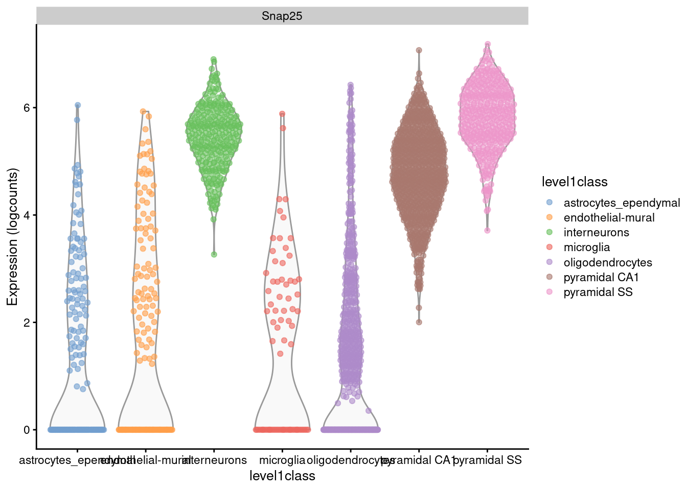
Figure 2.1: Distribution of log-expression values for Snap25 in each cell type of the Zeisel brain dataset.
Centering also allows us to interpret a pseudo-count of 1 as an extra read or UMI for each gene. In practical terms, this means that the shrinkage effect of the pseudo-count diminishes as read/UMI counts increase. As a result, any estimates of log-fold changes in expression (e.g., from differences in the log-values between groups of cells) become increasingly accurate with deeper coverage. Conversely, at lower counts, stronger shrinkage avoids inflated differences due to sampling noise, which might otherwise mask interesting features in downstream analyses like clustering. In some sense, the pseudo-count aims to protect later analyses from the lack of information at low counts while trying to miminize its own effect at high counts.
For comparison, consider the situation where we applied a constant pseudo-count to some count-per-million-like measure. It is easy to see that the accuracy of the subsequent log-fold changes would never improve regardless of how much additional sequencing was performed; scaling to a constant library size of a million means that the pseudo-count will have the same effect for all datasets. This is ironic given that the whole intention of sequencing more deeply is to improve quantification of these differences between cell subpopulations. The same criticism applies to popular metrics like the “counts-per-10K” used in, e.g., seurat.
2.3 Downsampling instead of scaling
In rare cases, direct scaling of the counts is not appropriate due to the effect described by A. Lun (2018). Briefly, this is caused by the fact that the mean of the log-normalized counts is not the same as the log-transformed mean of the normalized counts. The difference between them depends on the mean and variance of the original counts, such that there is a systematic trend in the mean of the log-counts with respect to the count size. This typically manifests as trajectories correlated strongly with library size even after library size normalization, as shown in Figure 2.2 for synthetic scRNA-seq data generated with a pool-and-split approach (Tian et al. 2019).
# TODO: move to scRNAseq.
library(BiocFileCache)
bfc <- BiocFileCache(ask=FALSE)
qcdata <- bfcrpath(bfc, "https://github.com/LuyiTian/CellBench_data/blob/master/data/mRNAmix_qc.RData?raw=true")

env <- new.env()
load(qcdata, envir=env)
sce.8qc <- env$sce8_qc

# Library size normalization and log-transformation.
sce.8qc <- logNormCounts(sce.8qc)
sce.8qc <- runPCA(sce.8qc)
gridExtra::grid.arrange(
    plotPCA(sce.8qc, colour_by=I(factor(sce.8qc$mix))),
    plotPCA(sce.8qc, colour_by=I(librarySizeFactors(sce.8qc))),
    ncol=2
)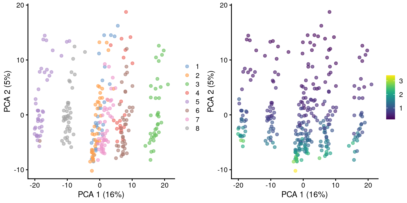
Figure 2.2: PCA plot of all pool-and-split libraries in the SORT-seq CellBench data, computed from the log-normalized expression values with library size-derived size factors. Each point represents a library and is colored by the mixing ratio used to construct it (left) or by the size factor (right).
As the problem arises from differences in the sizes of the counts, the most straightforward solution is to downsample the counts of the high-coverage cells to match those of low-coverage cells. This uses the size factors to determine the amount of downsampling for each cell required to reach the 1st percentile of size factors. (The small minority of cells with smaller size factors are simply scaled up. We do not attempt to downsample to the smallest size factor, as this would result in excessive loss of information for one aberrant cell with very low size factors.) We can see that this eliminates the library size factor-associated trajectories from the first two PCs, improving resolution of the known differences based on mixing ratios (Figure 2.3). The log-transformation is still necessary but no longer introduces a shift in the means when the sizes of the counts are similar across cells.
sce.8qc2 <- logNormCounts(sce.8qc, downsample=TRUE)
sce.8qc2 <- runPCA(sce.8qc2)
gridExtra::grid.arrange(
    plotPCA(sce.8qc2, colour_by=I(factor(sce.8qc2$mix))),
    plotPCA(sce.8qc2, colour_by=I(librarySizeFactors(sce.8qc2))),
    ncol=2
)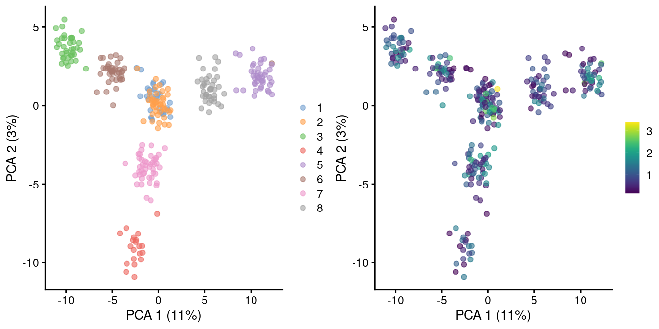
Figure 2.3: PCA plot of pool-and-split libraries in the SORT-seq CellBench data, computed from the log-transformed counts after downsampling in proportion to the library size factors. Each point represents a library and is colored by the mixing ratio used to construct it (left) or by the size factor (right).
While downsampling is an expedient solution, it is statistically inefficient as it needs to increase the noise of high-coverage cells in order to avoid differences with low-coverage cells. It is also slower than simple scaling. Thus, we would only recommend using this approach after an initial analysis with scaled counts reveals suspicious trajectories that are strongly correlated with the size factors. In such cases, it is a simple matter to re-normalize by downsampling to determine whether the trajectory is an artifact of the log-transformation.
2.5 Normalization versus batch correction
It is worth noting the difference between normalization and batch correction (Multi-sample Chapter 1). Normalization typically refers to removal of technical biases between cells, while batch correction involves removal of both technical biases and biological differences between batches. Technical biases are relatively simple and straightforward to remove, whereas biological differences between batches can be highly unpredictable. On the other hand, batch correction algorithms can share information between cells in the same batch, as all cells in the same batch are assumed to be subject to the same batch effect, whereas most normalization strategies tend to operate on a cell-by-cell basis with less information sharing.
The key point here is that normalization and batch correction are different tasks, involve different assumptions and generally require different computational methods (though some packages aim to perform both steps at once, e.g., zinbwave). Thus, it is important to distinguish between “normalized” and “batch-corrected” data, as these usually refer to different stages of processing. Of course, these processes are not exclusive, and most workflows will perform normalization within each batch followed by correction between batches. Interested readers are directed to Multi-sample Chapter 1 for more details.
Session Info
R version 4.1.0 (2021-05-18)
Platform: x86_64-pc-linux-gnu (64-bit)
Running under: Ubuntu 20.04.2 LTS

Matrix products: default
BLAS:   /home/biocbuild/bbs-3.13-bioc/R/lib/libRblas.so
LAPACK: /home/biocbuild/bbs-3.13-bioc/R/lib/libRlapack.so

locale:
 [1] LC_CTYPE=en_US.UTF-8       LC_NUMERIC=C
 [3] LC_TIME=en_US.UTF-8        LC_COLLATE=C
 [5] LC_MONETARY=en_US.UTF-8    LC_MESSAGES=en_US.UTF-8
 [7] LC_PAPER=en_US.UTF-8       LC_NAME=C
 [9] LC_ADDRESS=C               LC_TELEPHONE=C
[11] LC_MEASUREMENT=en_US.UTF-8 LC_IDENTIFICATION=C

attached base packages:
[1] parallel  stats4    stats     graphics  grDevices utils     datasets
[8] methods   base

other attached packages:
 [1] BiocFileCache_2.0.0         dbplyr_2.1.1
 [3] scater_1.20.0               ggplot2_3.3.3
 [5] scuttle_1.2.0               SingleCellExperiment_1.14.0
 [7] SummarizedExperiment_1.22.0 Biobase_2.52.0
 [9] GenomicRanges_1.44.0        GenomeInfoDb_1.28.0
[11] IRanges_2.26.0              S4Vectors_0.30.0
[13] BiocGenerics_0.38.0         MatrixGenerics_1.4.0
[15] matrixStats_0.58.0          BiocStyle_2.20.0
[17] rebook_1.2.0

loaded via a namespace (and not attached):
 [1] bitops_1.0-7              bit64_4.0.5
 [3] httr_1.4.2                filelock_1.0.2
 [5] tools_4.1.0               bslib_0.2.5.1
 [7] utf8_1.2.1                R6_2.5.0
 [9] irlba_2.3.3               vipor_0.4.5
[11] DBI_1.1.1                 colorspace_2.0-1
[13] withr_2.4.2               tidyselect_1.1.1
[15] gridExtra_2.3             curl_4.3.1
[17] bit_4.0.4                 compiler_4.1.0
[19] graph_1.70.0              BiocNeighbors_1.10.0
[21] DelayedArray_0.18.0       labeling_0.4.2
[23] bookdown_0.22             sass_0.4.0
[25] scales_1.1.1              rappdirs_0.3.3
[27] stringr_1.4.0             digest_0.6.27
[29] rmarkdown_2.8             XVector_0.32.0
[31] pkgconfig_2.0.3           htmltools_0.5.1.1
[33] sparseMatrixStats_1.4.0   fastmap_1.1.0
[35] highr_0.9                 rlang_0.4.11
[37] RSQLite_2.2.7             DelayedMatrixStats_1.14.0
[39] farver_2.1.0              jquerylib_0.1.4
[41] generics_0.1.0            jsonlite_1.7.2
[43] BiocParallel_1.26.0       dplyr_1.0.6
[45] RCurl_1.98-1.3            magrittr_2.0.1
[47] BiocSingular_1.8.0        GenomeInfoDbData_1.2.6
[49] Matrix_1.3-3              Rcpp_1.0.6
[51] ggbeeswarm_0.6.0          munsell_0.5.0
[53] fansi_0.4.2               viridis_0.6.1
[55] lifecycle_1.0.0           stringi_1.6.2
[57] yaml_2.2.1                zlibbioc_1.38.0
[59] blob_1.2.1                grid_4.1.0
[61] crayon_1.4.1              dir.expiry_1.0.0
[63] lattice_0.20-44           cowplot_1.1.1
[65] beachmat_2.8.0            CodeDepends_0.6.5
[67] knitr_1.33                pillar_1.6.1
[69] codetools_0.2-18          ScaledMatrix_1.0.0
[71] XML_3.99-0.6              glue_1.4.2
[73] evaluate_0.14             BiocManager_1.30.15
[75] vctrs_0.3.8               gtable_0.3.0
[77] purrr_0.3.4               assertthat_0.2.1
[79] cachem_1.0.5              xfun_0.23
[81] rsvd_1.0.5                viridisLite_0.4.0
[83] tibble_3.1.2              memoise_2.0.0
[85] beeswarm_0.3.1            ellipsis_0.3.2
References
Lun, A. 2018. “Overcoming Systematic Errors Caused by Log-Transformation of Normalized Single-Cell Rna Sequencing Data.” bioRxiv.
Tian, L., X. Dong, S. Freytag, K. A. Le Cao, S. Su, A. JalalAbadi, D. Amann-Zalcenstein, et al. 2019. “Benchmarking single cell RNA-sequencing analysis pipelines using mixture control experiments.” Nat. Methods 16 (6): 479–87.
2.4 Comments on other transformations
Of course, the log-transformation is not the only possible transformation. Another somewhat common choice is the square root, motivated by the fact that it is the variance stabilizing transformation for Poisson-distributed counts. This assumes that counts are actually Poisson-distributed, which is true enough from the perspective of sequencing noise in UMI counts but ignores biological overdispersion. One may also see the inverse hyperbolic sine (a.k.a, arcsinh) transformation being used on occasion, which is very similar to the log-transformation when considering non-negative values. The main practical difference for scRNA-seq applications is a larger initial jump from zero to non-zero values.
Alternatively, we may use more sophisticated approaches for variance stabilizing transformations in genomics data, e.g., DESeq2 or sctransform. These aim to remove the mean-variance trend more effectively than the simpler transformations mentioned above, though it could be argued whether this is actually desirable. For low-coverage scRNA-seq data, there will always be a mean-variance trend under any transformation, for the simple reason that the variance must be zero when the mean count is zero. These methods also face the challenge of removing the mean-variance trend while preserving the interesting component of variation, i.e., the log-fold changes between subpopulations; this may or may not be done adequately, depending on the aggressiveness of the algorithm.
In practice, the log-transformation is a good default choice due to its simplicity and interpretability, and is what we will be using for all downstream analyses.