ApoAI Data:
Two groups compared through a common reference
Gordon Smyth
16 August 2005
1. Aims
This case study introduces linear modeling as a tool for identifying differentially express genes in the context of a two-group cDNA microarray experiment using a common reference.
2. Required data
The ApoAI data set is required for this lab and can be obtained from apoai.zip. You should create a clean directory, unpack this file into that directory, then set that directory as your working directory for your R session using setwd() or otherwise.
3. The ApoAI experiment
In this section we consider a case study where two
RNA sources are compared through a common reference
RNA. The analysis of the log-ratios involves a
two-sample comparison of means for each gene. The data
is available as an RGList object in the saved R data
file ApoAI.RData.
Background. The data is from a study of lipid metabolism by Callow et al (2000). The apolipoprotein AI (ApoAI) gene is known to play a pivotal role in high density lipoprotein (HDL) metabolism. Mice which have the ApoAI gene knocked out have very low HDL cholesterol levels. The purpose of this experiment is to determine how ApoAI deficiency affects the action of other genes in the liver, with the idea that this will help determine the molecular pathways through which ApoAI operates.
Hybridizations. The experiment compared 8 ApoAI knockout mice with 8 wild type (normal) C57BL/6 ("black six") mice, the control mice. For each of these 16 mice, target mRNA was obtained from liver tissue and labelled using a Cy5 dye. The RNA from each mouse was hybridized to a separate microarray. Common reference RNA was labelled with Cy3 dye and used for all the arrays. The reference RNA was obtained by pooling RNA extracted from the 8 control mice.
| Number of arrays | Red (Cy5) | Green (Cy3) |
|---|---|---|
| 8 | Wild Type "black six" mice (WT) | Pooled Reference (Ref) |
| 8 | ApoAI Knockout (KO) | Pooled Reference (Ref) |
Diagrammatically, the experimental design is:
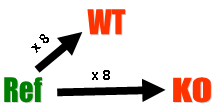
This is an example of a single comparison experiment using a common reference. The fact that the comparison is made by way of a common reference rather than directly as for the swirl experiment makes this, for each gene, a two-sample rather than a single-sample setup.
4. Load the data
 library(limma)
 load("ApoAI.RData")
 objects()
 names(RG)
 RG$targets
 RG
Exercise: All data objects in limma have object-orientated features which allow them to behave in many ways, such as subsetting, cbind() and rbind(), analogously to ordinary matrices. Explore the matrix-like properties of RGList objects. Try for example:
 dim(RG)
 ncol(RG)
 colnames(RG)
 RG[,1:2]
 RG1 <- RG[,1:2]
 RG2 <- RG[,9:10]
 cbind(RG1,RG2)
 i <- RG$genes$TYPE=="Control"
 RG[i,]
5. Normalize
The following command does print-tip loess normalization of the log-ratios by default:
MA <- normalizeWithinArrays(RG)
6. Defining a design matrix
In order to construct a design matrix, let us remind ourselves of the linear model which we are fitting for each gene:
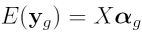
where  is the vector of normalized log
ratios from the sixteen arrays,
is the vector of normalized log
ratios from the sixteen arrays,  is the Expected Value of ,
  is
the design matrix and
is
the design matrix and  is the vector of log ratios to estimate,
corresponding to the "M" (fold change) column in
the final list of differentially expressed genes given
by
is the vector of log ratios to estimate,
corresponding to the "M" (fold change) column in
the final list of differentially expressed genes given
by topTable(). The estimated log ratios
are also known as "coefficients", "parameters" and "log
fold changes".
This experiment has three types of RNA: Reference
(Ref), Wild Type (WT), and Knockout
(KO), so it is sufficient to estimate two log
ratios in the linear model for each gene, i.e. we will
estimate two parameters, so our design matrix should
have two columns. In our case, the two parameters in
the vector are the log ratios which
compare gene expression levels in WT vs Ref and
KO vs WT. (There are other possible
parameterizations which could have been chosen instead.
We are using one which allows us to estimate the
contrast of interest (KO vs WT) directly from
the linear model fit, rather than estimating it later
as a contrast (i.e. a linear combination of parameters
estimated from the linear model).
The design matrix we will use is:
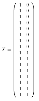
where the first column is for the "WT vs Ref" parameter and the second column is for the "KO vs WT" parameter. The first 8 arrays hybridize WT RNA with Ref RNA so it makes sense that they each have a '1' in the WT vs Ref column. The last 8 arrays hybridize KO RNA with Ref RNA which corresponds to the sum of the two parameters, "WT vs Ref" and "KO vs WT" which is clear if you replace "vs" with a minus sign (remembering that everything has been log2 transformed so that subtraction here actually represents a log ratio).
This design matrix can be defined in R as follows:
 design <- cbind("WT-Ref"=1,"KO-WT"=rep(0:1,c(8,8)))
 design
Exercise: Find another way to construct this same design matrix using RG$targets$Cy5 and model.matrix().
7. Fitting a linear model
 fit <- lmFit(MA,design=design)
 colnames(fit)
 names(fit)
8. Empirical Bayes statistics
 fit <- eBayes(fit)
 names(fit)
 summary(fit)
9. Display tables of differentially expressed genes
We now use the function topTable to
obtain a list the genes with the most evidence of
differential expression between the Knockout and
Wild-Type RNA samples. The knockout gene (ApoAI) should
theoretically have a log fold change of minus infinity,
but microarrays cannot measure extremely large fold
changes. While the M value of the ApoAI gene in the
topTable may not have much biological meaning, the high
ranking shows that this gene is consistently
down-regulated across the replicate arrays.
topTable(fit,coef="KO-WT",adjust="fdr")The arguments of topTable can be studied in more detail with
?topTable or args(topTable). The default
method for ranking genes is the B statistic (log odds of
differential expression, Lonnstedt and Speed [2]), but the
moderated t statistic and p-value can also be used. Using the
average fold-change (the M column) is not usually recommended
because this ignores the genewise variability between replicate
arrays.
Exercise: Try to achieve the same top-table using a completely different design matrix and forming contrasts. Use the function
modelMatrix(RG$targets, ref="Pool")
to format a different design matrix. Then use makeContrasts() and contrasts.fit() to form the KO vs Wt comparison.
10. Removing control spots
In most practical studies one will want to remove the control probes from the data before undertaking the differential expression study. This can be done by examining the columns of the probe annotation data frame, RG$genes:
 table(RG$genes$TYPE)
 isGene <- RG$genes$TYPE=="cDNA"
 MA2 <- MA[isGene,]
Now repeat the linear model steps with the reduced data.
11. MA plot of coefficients from the fitted model
Using an M A plot, we can see which genes are selected as being differentially expressed by the B statistic (log odds of differential expression), which is the default ranking statistic for the topTable. Of course, the differentially expressed genes selected by the B statistic may not have the most extreme fold changes (M values), because some of the genes with extreme average fold changes may vary significantly between replicate arrays so they will be down-weighted by the empirical Bayes statistics.
plotMA(fit, 2)
Now add gene labels:
 top10 <- order(fit$lods[,"KO-WT"],decreasing=TRUE)[1:10]
 A <- fit$Amean
 M <- fit$coef[,2]
 shortlabels <- substring(fit$genes[,"NAME"],1,5)
 text(A[top10],M[top10],labels=shortlabels[top10],cex=0.8,col="blue")
Acknowledgements
Thanks to Yee Hwa Yang and Sandrine Dudoit for the ApoAI data.
References
- Callow, M. J., Dudoit, S., Gong, E. L., Speed, T. P., and Rubin, E. M. (2000). Microarray expression profiling identifies genes with altered expression in HDL deficient mice. Genome Research 10, 2022-2029. http://www.genome.org/cgi/content/full/10/12/2022
- Smyth, G. K., and Speed, T. P. (2003). Normalization of cDNA microarray data. Methods 31, 265-273. http://www.statsci.org/smyth/pubs/normalize.pdf
- L�nnstedt, I, and Speed T. P. (2002). Replicated microarray data. Statistica Sinica 12, 31-46.
- Smyth, G. K. (2004). Linear models and empirical Bayes methods for assessing differential expression in microarray experiments. Statistical Applications in Genetics and Molecular Biology 3, No. 1, Article 3. http://www.bepress.com/sagmb/vol3/iss1/art3/
Glossary
| Knockout RNA | RNA extracted from a biological specimen which has had one gene artificially knocked out (removed) from it in a laboratory. |
| Wild Type RNA | RNA extracted from a biological specimen whose genes are in their natural form (as found in the wild). |