Chapter 5 Using multiple references
5.1 Overview
In some cases, we may wish to use multiple references for annotation of a test dataset. This yields a more comprehensive set of cell types that are not covered by any individual reference, especially when differences in the resolution are considered. However, it is not trivial due to the presence of batch effects across references (from differences in technology, experimental protocol or the biological system) as well as differences in the annotation vocabulary between investigators.
Several strategies are available to combine inferences from multiple references:
- using reference-specific labels in a combined reference
- using harmonized labels in a combined reference
- combining scores across multiple references
This chapter discusses the various strengths and weaknesses of each strategy and provides some practical demonstrations of each. Here, we will use the HPCA and Blueprint/ENCODE datasets as our references and (yet another) PBMC dataset as the test.
5.2 Using reference-specific labels
In this strategy, each label is defined in the context of its reference dataset. This means that a label - say, “B cell” - in reference dataset X is considered to be different from a “B cell” label in reference dataset Y. Use of reference-specific labels is most appropriate if there are relevant biological differences between the references; for example, if one reference is concerned with healthy tissue while the other reference considers diseased tissue, it can be helpful to distinguish between the same cell type in different biological contexts.
We can easily implement this approach by combining the expression matrices together
and pasting the reference name onto the corresponding character vector of labels.
This modification ensures that the downstream SingleR() call
will treat each label-reference combination as a distinct entity.
hpca2 <- hpca
hpca2$label.main <- paste0("HPCA.", hpca2$label.main)

bpe2 <- bpe
bpe2$label.main <- paste0("BPE.", bpe2$label.main)

shared <- intersect(rownames(hpca2), rownames(bpe2))
combined <- cbind(hpca2[shared,], bpe2[shared,])
It is then straightforward to perform annotation with the usual methods.
library(SingleR)
com.res1 <- SingleR(pbmc, ref=combined, labels=combined$label.main, assay.type.test=1)
table(com.res1$labels)
##
## BPE.B-cells BPE.CD4+ T-cells BPE.CD8+ T-cells BPE.HSC
## 1178 1708 2656 20
## BPE.Monocytes BPE.NK cells HPCA.HSC_-G-CSF HPCA.Platelets
## 2349 460 1 7
## HPCA.T_cells
## 2However, this strategy identifies markers by directly comparing expression values across references, meaning that the marker set is likely to contain genes responsible for uninteresting batch effects. This will increase noise during the calculation of the score in each reference, possibly leading to a loss of precision and a greater risk of technical variation dominating the classification results. The use of reference-specific labels also complicates interpretation of the results as the cell type is always qualified by its reference of origin.
5.3 Comparing scores across references
5.3.1 Combining inferences from individual references
Another strategy - and the default approach implemented in SingleR() -
involves performing classification separately within each reference,
and then collating the results to choose the label with the highest score across references.
This is a relatively expedient approach that avoids the need for explicit harmonization
while also reducing exposure to reference-specific batch effects.
To use this method, we simply pass multiple objects to the ref= and label= argument in SingleR().
The combining strategy is as follows:
- The function first annotates the test dataset with each reference individually
in the same manner as described in Section 1.2.
This step is almost equivalent to simply looping over all individual references and running
SingleR()on each. - For each cell, the function collects its predicted labels across all references. In doing so, it also identifies the union of markers that are upregulated in the predicted label in each reference.
- The function identifies the overall best-scoring label as the final prediction for that cell. This step involves a recomputation of the scores across the identified marker subset to ensure that these scores are derived from the same set of genes (and are thus comparable across references).
The function will then return a DataFrame of combined results for each cell in the test dataset,
including the overall label and the reference from which it was assigned.
com.res2 <- SingleR(test = pbmc, assay.type.test=1,
    ref = list(BPE=bpe, HPCA=hpca),
    labels = list(bpe$label.main, hpca$label.main))

# Check the final label from the combined assignment.
table(com.res2$labels)
##
## B-cells B_cell CD4+ T-cells CD8+ T-cells
## 1170 14 1450 2936
## GMP HSC Monocyte Monocytes
## 1 22 753 1560
## NK cells NK_cell Platelets Pre-B_cell_CD34-
## 372 10 9 16
## T_cells
## 68##
## 1 2
## 7510 871The main appeal of this approach lies in the fact that it is based on the results of annotation with individual references. This avoids batch effects from comparing expression values across references; it reduces the need for any coordination in the label scheme between references; and simultaneously provides the per-reference annotations in the results. The last feature is particularly useful as it allows for more detailed diagnostics, troubleshooting and further analysis.
## [1] "B-cells"      "Monocytes"    "CD8+ T-cells" "CD8+ T-cells" "Monocytes"
## [6] "Monocytes"## [1] "B_cell" "Monocyte" "T_cells" "T_cells" "Monocyte" "Monocyte"The main downside is that it is somewhat suboptimal if there are many labels that are unique to one reference, as markers are not identified with the aim of distinguishing a label in one reference from another label in another reference. The continued lack of consistency in the labels across references also complicates interpretation of the results, though we can overcome this by using harmonized labels as described below.
5.3.2 Combined diagnostics
All of the diagnostic plots in SingleR will naturally operate on these combined results.
For example, we can create a heatmap of the scores in all of the individual references
as well as for the recomputed scores in the combined results (Figure 5.1).
Note that scores are only recomputed for the labels predicted in the individual references,
so all labels outside of those are simply set to NA - hence the swathes of grey.
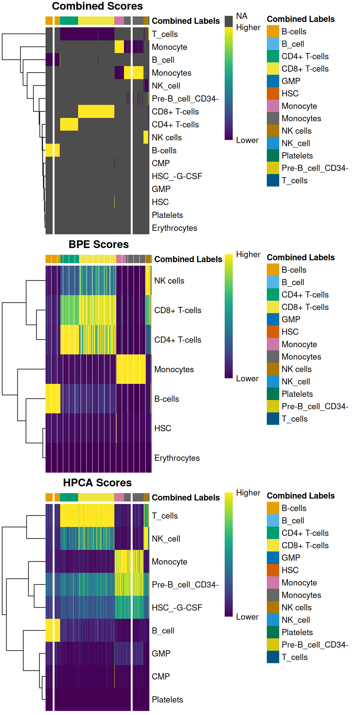
Figure 5.1: Heatmaps of assignment scores for each cell in the PBMC test dataset after being assigned to the Blueprint/ENCODE and Human Primary Cell Atlas reference datasets. One heatmap is shown for the recomputed scores and the scores from each individual reference. The annotation at the top of each heatmap represents the final combined prediction for each cell.
The deltas for each individual reference can also be plotted with plotDeltaDistribution() (Figure 5.2).
No deltas are shown for the recomputed scores as the assumption described in Section 4.3
may not be applicable across the predicted labels from the individual references.
For example, if all individual references suggest the same cell type with similar recomputed scores,
any delta would be low even though the assignment is highly confident.
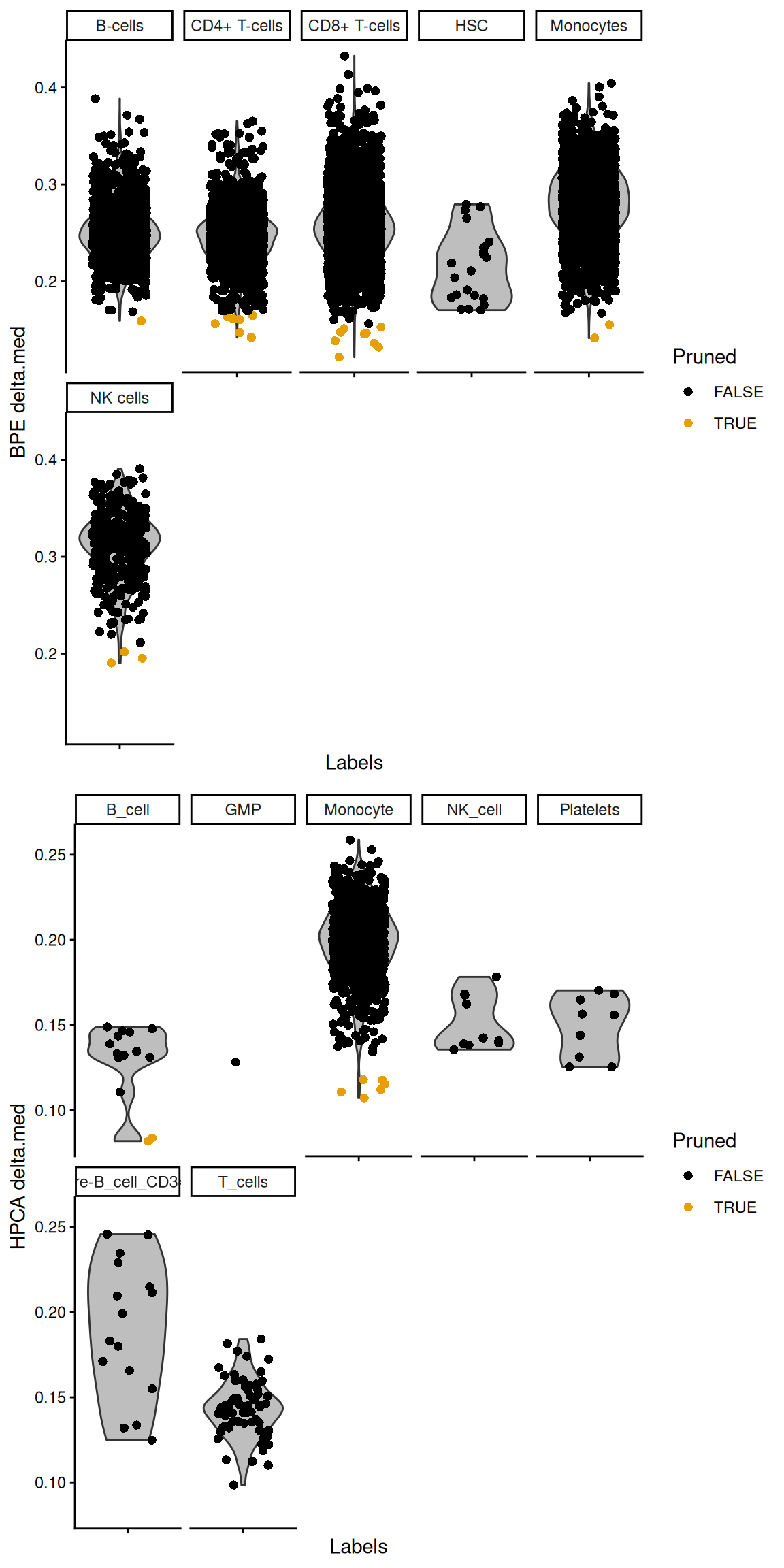
Figure 5.2: Distribution of the deltas across cells in the PBMC test dataset for each label in the Blueprint/ENCODE and Human Primary Cell Atlas reference datasets. Each point represents a cell that was assigned to that label in the combined results, colored by whether it was pruned or not in the corresponding individual reference.
We can similarly extract marker genes to use in heatmaps as described in Section 4.4.
As annotation was performed to each individual reference,
we can simply extract the marker genes from the nested DataFrames as shown in Figure 5.3.
hpca.markers <- metadata(com.res2$orig.results$HPCA)$de.genes
bpe.markers <- metadata(com.res2$orig.results$BPE)$de.genes
mono.markers <- unique(unlist(c(hpca.markers$Monocyte, bpe.markers$Monocytes)))

library(scater)
plotHeatmap(logNormCounts(pbmc),
    order_columns_by=list(I(com.res2$labels)),
    features=mono.markers)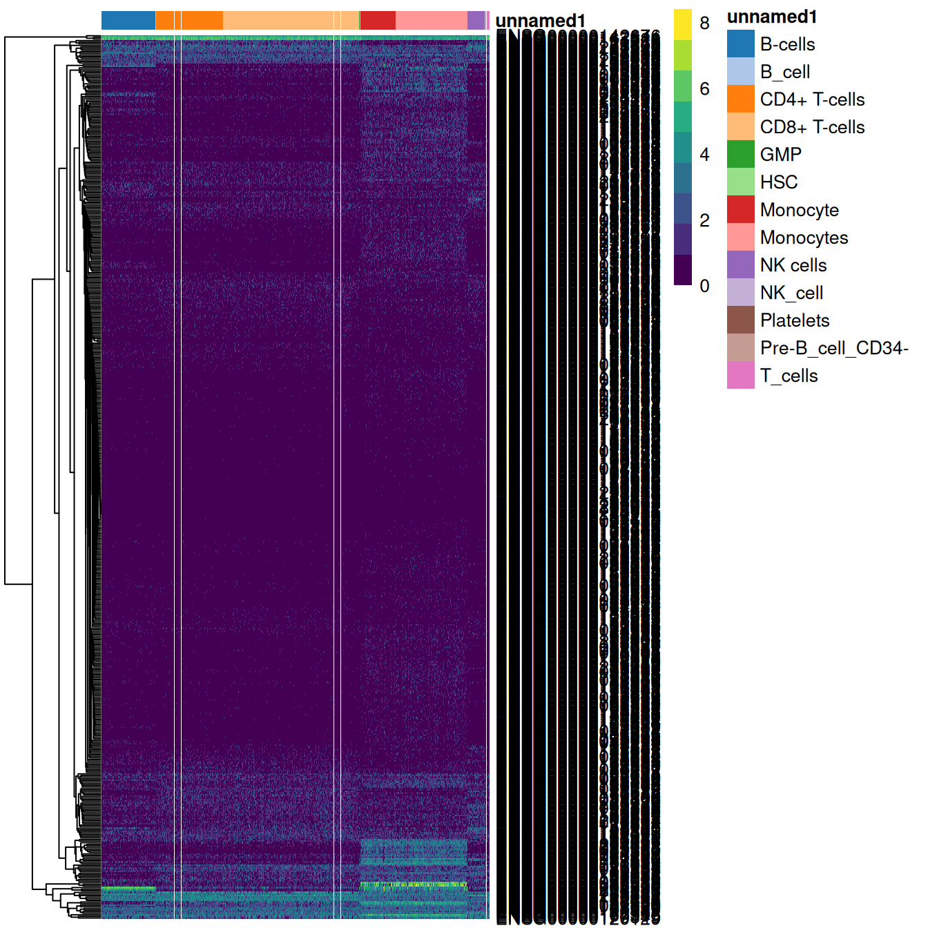
Figure 5.3: Heatmap of log-expression values in the PBMC dataset for all marker genes upregulated in monocytes in the Blueprint/ENCODE and Human Primary Cell Atlas reference datasets. Combined labels for each cell are shown at the top.
5.4 Using harmonized labels
5.4.2 Manual label harmonization
The matchReferences() function provides a simple approach for label harmonization between two references.
Each reference is used to annotate the other and the probability of mutual assignment between each pair of labels is computed,
i.e., for each pair of labels, what is the probability that a cell with one label is assigned the other and vice versa?
Probabilities close to 1 in Figure 5.4 indicate there is a 1:1 relation between that pair of labels;
on the other hand, an all-zero probability vector indicates that a label is unique to a particular reference.
library(SingleR)
bp.se <- BlueprintEncodeData()
hpca.se <- HumanPrimaryCellAtlasData()

matched <- matchReferences(bp.se, hpca.se,
    bp.se$label.main, hpca.se$label.main)
pheatmap::pheatmap(matched, col=viridis::plasma(100))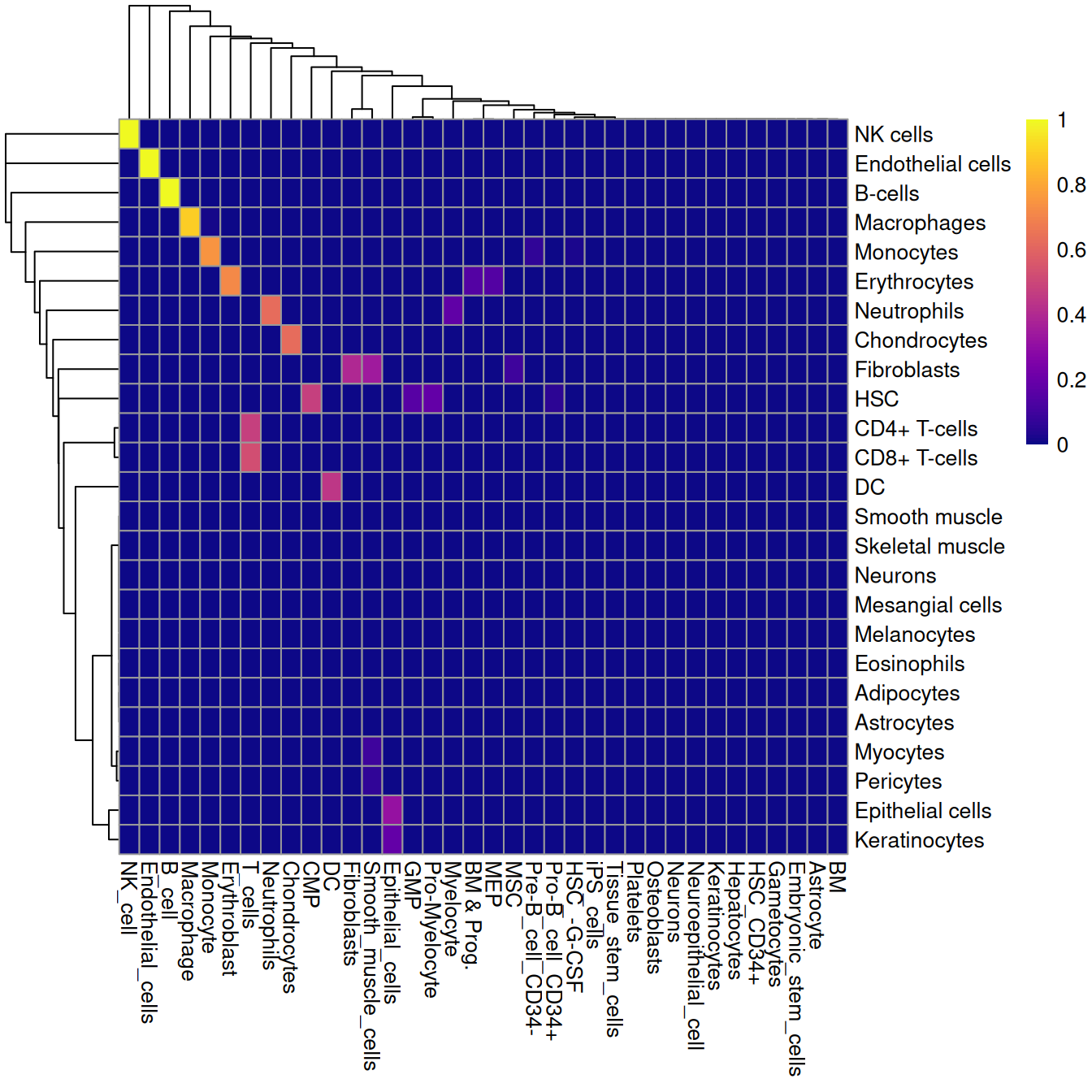
Figure 5.4: Heatmap of mutual assignment probabilities between the Blueprint/ENCODE reference dataset (labels in rows) and the Human primary cell atlas reference (labels in columns).
This function can be used to guide harmonization to enforce a consistent vocabulary between two sets of labels. However, some manual intervention is still required in this process given the ambiguities posed by differences in biological systems and technologies. In the example above, neurons are considered to be unique to each reference while smooth muscle cells in the HPCA data are incorrectly matched to fibroblasts in the Blueprint/ENCODE data. CD4+ and CD8+ T cells are also both assigned to “T cells”, so some decision about the acceptable resolution of the harmonized labels is required here.
As an aside, we can also use this function to identify the matching clusters between two independent scRNA-seq analyses. This involves substituting the cluster assignments as proxies for the labels, allowing us to match up clusters and integrate conclusions from multiple datasets without the difficulties of batch correction and reclustering.
Session info
R version 4.6.0 RC (2026-04-17 r89917)
Platform: x86_64-pc-linux-gnu
Running under: Ubuntu 24.04.4 LTS

Matrix products: default
BLAS:   /home/biocbuild/bbs-3.23-bioc/R/lib/libRblas.so
LAPACK: /usr/lib/x86_64-linux-gnu/lapack/liblapack.so.3.12.0  LAPACK version 3.12.0

locale:
 [1] LC_CTYPE=en_US.UTF-8       LC_NUMERIC=C
 [3] LC_TIME=en_GB              LC_COLLATE=C
 [5] LC_MONETARY=en_US.UTF-8    LC_MESSAGES=en_US.UTF-8
 [7] LC_PAPER=en_US.UTF-8       LC_NAME=C
 [9] LC_ADDRESS=C               LC_TELEPHONE=C
[11] LC_MEASUREMENT=en_US.UTF-8 LC_IDENTIFICATION=C

time zone: America/New_York
tzcode source: system (glibc)

attached base packages:
[1] stats4    stats     graphics  grDevices utils     datasets  methods
[8] base

other attached packages:
 [1] scater_1.40.0               ggplot2_4.0.3
 [3] scuttle_1.22.0              SingleR_2.14.0
 [5] ensembldb_2.36.0            AnnotationFilter_1.36.0
 [7] GenomicFeatures_1.64.0      AnnotationDbi_1.74.0
 [9] celldex_1.21.0              TENxPBMCData_1.29.0
[11] HDF5Array_1.40.0            h5mread_1.4.0
[13] rhdf5_2.56.0                DelayedArray_0.38.0
[15] SparseArray_1.12.0          S4Arrays_1.12.0
[17] abind_1.4-8                 Matrix_1.7-5
[19] SingleCellExperiment_1.34.0 SummarizedExperiment_1.42.0
[21] Biobase_2.72.0              GenomicRanges_1.64.0
[23] Seqinfo_1.2.0               IRanges_2.46.0
[25] S4Vectors_0.50.0            BiocGenerics_0.58.0
[27] generics_0.1.4              MatrixGenerics_1.24.0
[29] matrixStats_1.5.0           BiocStyle_2.40.0
[31] rebook_1.22.0

loaded via a namespace (and not attached):
  [1] RColorBrewer_1.1-3        jsonlite_2.0.0
  [3] CodeDepends_0.6.7         magrittr_2.0.5
  [5] ggbeeswarm_0.7.3          gypsum_1.8.0
  [7] farver_2.1.2              rmarkdown_2.31
  [9] BiocIO_1.22.0             vctrs_0.7.3
 [11] memoise_2.0.1             Rsamtools_2.28.0
 [13] DelayedMatrixStats_1.34.0 RCurl_1.98-1.18
 [15] htmltools_0.5.9           AnnotationHub_4.2.0
 [17] curl_7.1.0                BiocNeighbors_2.6.0
 [19] Rhdf5lib_2.0.0            sass_0.4.10
 [21] alabaster.base_1.12.0     bslib_0.10.0
 [23] httr2_1.2.2               cachem_1.1.0
 [25] GenomicAlignments_1.48.0  lifecycle_1.0.5
 [27] pkgconfig_2.0.3           rsvd_1.0.5
 [29] R6_2.6.1                  fastmap_1.2.0
 [31] digest_0.6.39             irlba_2.3.7
 [33] ExperimentHub_3.2.0       RSQLite_2.4.6
 [35] beachmat_2.28.0           filelock_1.0.3
 [37] labeling_0.4.3            httr_1.4.8
 [39] compiler_4.6.0            bit64_4.8.0
 [41] withr_3.0.2               S7_0.2.2
 [43] BiocParallel_1.46.0       viridis_0.6.5
 [45] DBI_1.3.0                 alabaster.ranges_1.12.0
 [47] alabaster.schemas_1.12.0  rappdirs_0.3.4
 [49] rjson_0.2.23              tools_4.6.0
 [51] vipor_0.4.7               otel_0.2.0
 [53] beeswarm_0.4.0            glue_1.8.1
 [55] restfulr_0.0.16           rhdf5filters_1.24.0
 [57] grid_4.6.0                gtable_0.3.6
 [59] ScaledMatrix_1.20.0       BiocSingular_1.28.0
 [61] XVector_0.52.0            ggrepel_0.9.8
 [63] BiocVersion_3.23.1        pillar_1.11.1
 [65] dplyr_1.2.1               BiocFileCache_3.2.0
 [67] lattice_0.22-9            rtracklayer_1.72.0
 [69] bit_4.6.0                 tidyselect_1.2.1
 [71] Biostrings_2.80.0         knitr_1.51
 [73] gridExtra_2.3             bookdown_0.46
 [75] ProtGenerics_1.44.0       xfun_0.57
 [77] pheatmap_1.0.13           UCSC.utils_1.8.0
 [79] lazyeval_0.2.3            yaml_2.3.12
 [81] evaluate_1.0.5            codetools_0.2-20
 [83] cigarillo_1.2.0           tibble_3.3.1
 [85] alabaster.matrix_1.12.0   BiocManager_1.30.27
 [87] graph_1.90.0              cli_3.6.6
 [89] jquerylib_0.1.4           dichromat_2.0-0.1
 [91] Rcpp_1.1.1-1.1            GenomeInfoDb_1.48.0
 [93] dir.expiry_1.20.0         dbplyr_2.5.2
 [95] png_0.1-9                 XML_3.99-0.23
 [97] parallel_4.6.0            blob_1.3.0
 [99] beachmat.hdf5_1.10.0      sparseMatrixStats_1.24.0
[101] bitops_1.0-9              alabaster.se_1.12.0
[103] viridisLite_0.4.3         scales_1.4.0
[105] purrr_1.2.2               crayon_1.5.3
[107] rlang_1.2.0               KEGGREST_1.52.0