Chapter 7 Lawlor human pancreas (SMARTer)
7.1 Introduction
This performs an analysis of the Lawlor et al. (2017) dataset, consisting of human pancreas cells from various donors.
7.3 Quality control
library(scater)
stats <- perCellQCMetrics(sce.lawlor,
    subsets=list(Mito=which(rowData(sce.lawlor)$SEQNAME=="MT")))
qc <- quickPerCellQC(stats, percent_subsets="subsets_Mito_percent",
    batch=sce.lawlor$`islet unos id`)
sce.lawlor <- sce.lawlor[,!qc$discard]colData(unfiltered) <- cbind(colData(unfiltered), stats)
unfiltered$discard <- qc$discard
gridExtra::grid.arrange(
plotColData(unfiltered, x="islet unos id", y="sum", colour_by="discard") +
scale_y_log10() + ggtitle("Total count") +
theme(axis.text.x = element_text(angle = 90)),
plotColData(unfiltered, x="islet unos id", y="detected",
colour_by="discard") + scale_y_log10() + ggtitle("Detected features") +
theme(axis.text.x = element_text(angle = 90)),
plotColData(unfiltered, x="islet unos id", y="subsets_Mito_percent",
colour_by="discard") + ggtitle("Mito percent") +
theme(axis.text.x = element_text(angle = 90)),
ncol=2
)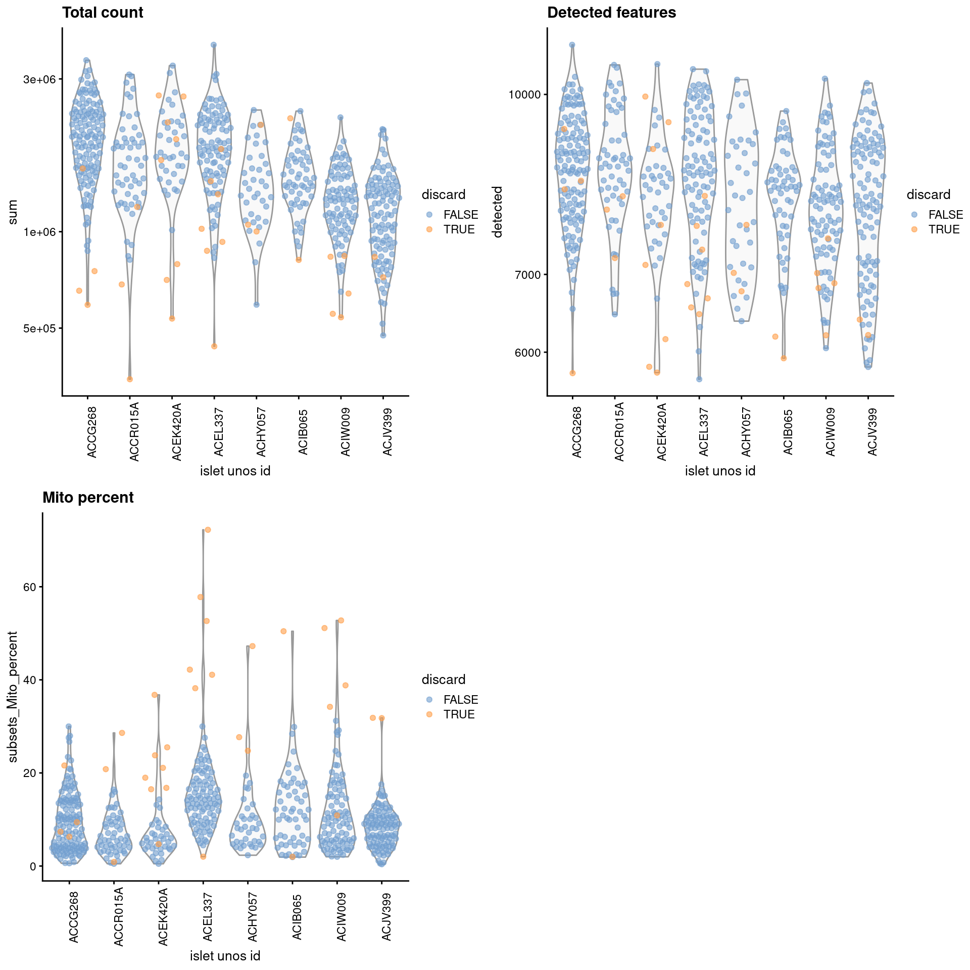
Figure 7.1: Distribution of each QC metric across cells from each donor of the Lawlor pancreas dataset. Each point represents a cell and is colored according to whether that cell was discarded.
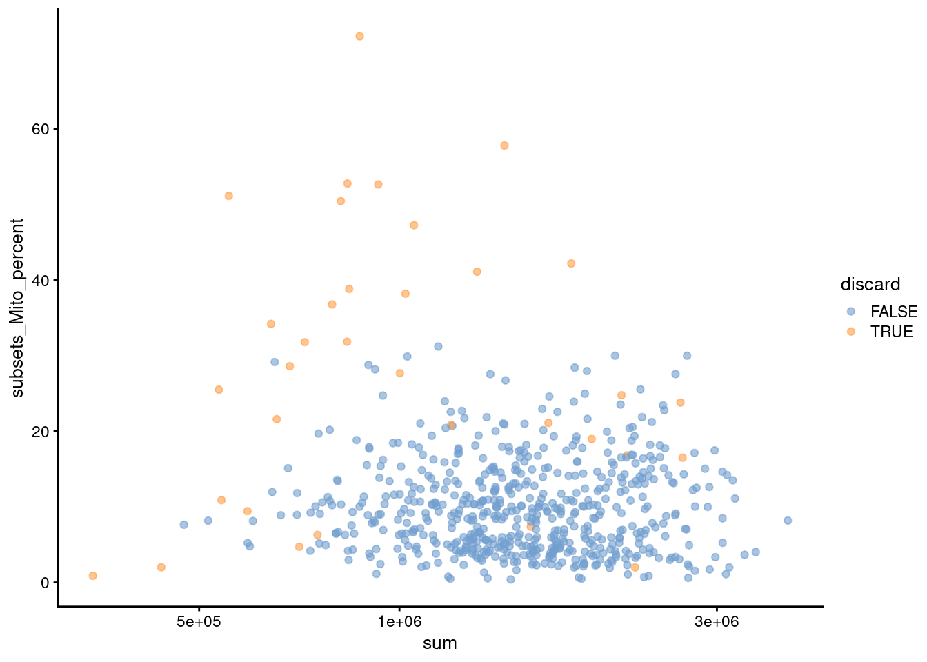
Figure 7.2: Percentage of mitochondrial reads in each cell in the 416B dataset compared to the total count. Each point represents a cell and is colored according to whether that cell was discarded.
##              low_lib_size            low_n_features high_subsets_Mito_percent
##                         9                         5                        25
##                   discard
##                        34
7.4 Normalization
library(scran)
set.seed(1000)
clusters <- quickCluster(sce.lawlor)
sce.lawlor <- computeSumFactors(sce.lawlor, clusters=clusters)
sce.lawlor <- logNormCounts(sce.lawlor)## Min. 1st Qu. Median Mean 3rd Qu. Max.
## 0.295 0.781 0.963 1.000 1.182 2.629plot(librarySizeFactors(sce.lawlor), sizeFactors(sce.lawlor), pch=16,
xlab="Library size factors", ylab="Deconvolution factors", log="xy")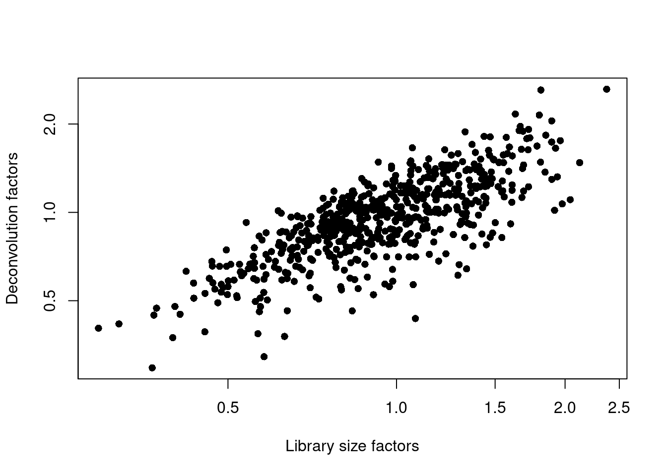
Figure 7.3: Relationship between the library size factors and the deconvolution size factors in the Lawlor pancreas dataset.
7.5 Variance modelling
Using age as a proxy for the donor.
dec.lawlor <- modelGeneVar(sce.lawlor, block=sce.lawlor$`islet unos id`)
chosen.genes <- getTopHVGs(dec.lawlor, n=2000)par(mfrow=c(4,2))
blocked.stats <- dec.lawlor$per.block
for (i in colnames(blocked.stats)) {
current <- blocked.stats[[i]]
plot(current$mean, current$total, main=i, pch=16, cex=0.5,
xlab="Mean of log-expression", ylab="Variance of log-expression")
curfit <- metadata(current)
curve(curfit$trend(x), col='dodgerblue', add=TRUE, lwd=2)
}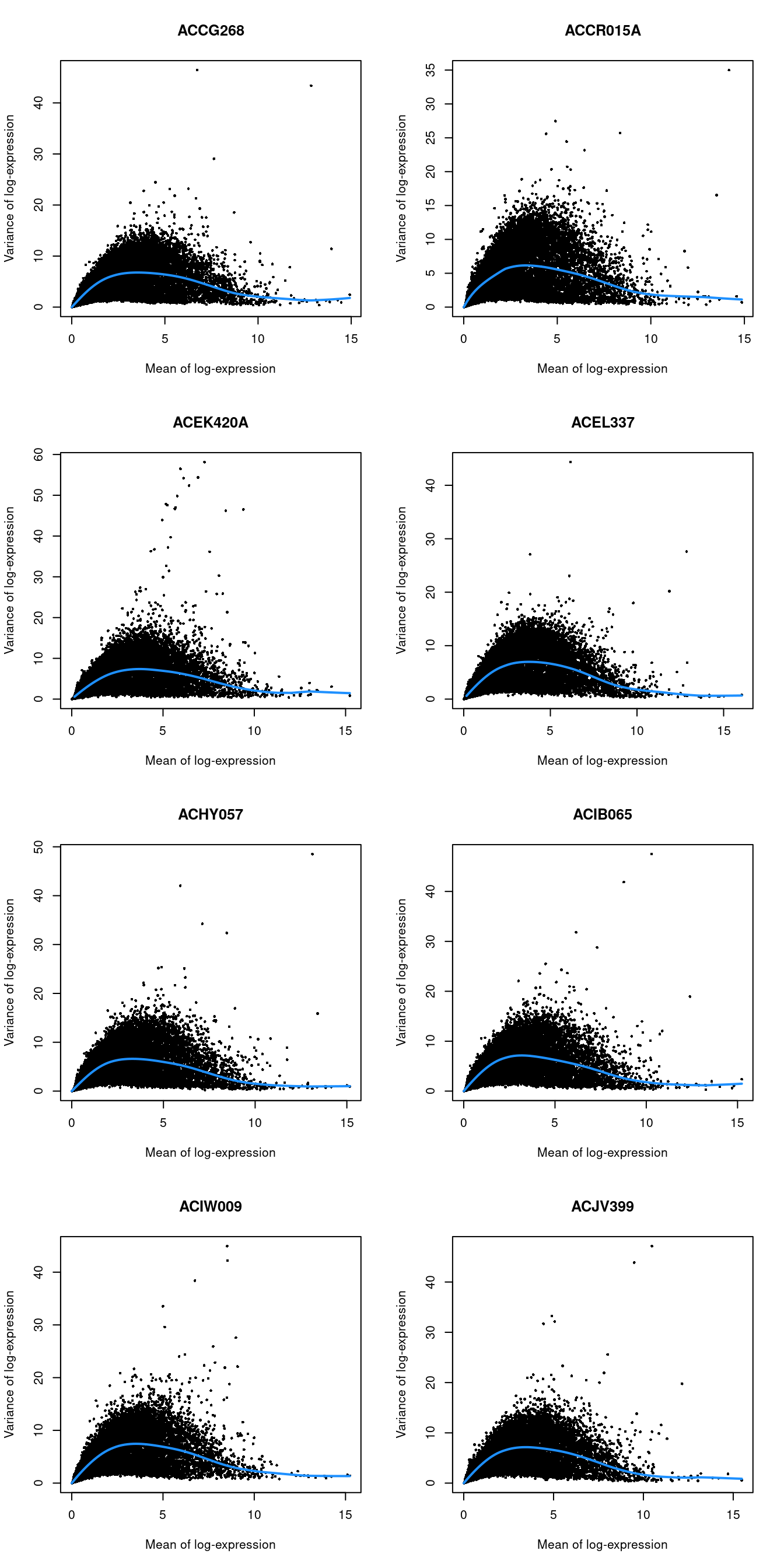
Figure 7.4: Per-gene variance as a function of the mean for the log-expression values in the Lawlor pancreas dataset. Each point represents a gene (black) with the mean-variance trend (blue) fitted separately for each donor.
7.7 Clustering
snn.gr <- buildSNNGraph(sce.lawlor, use.dimred="PCA")
colLabels(sce.lawlor) <- factor(igraph::cluster_walktrap(snn.gr)$membership)##
## Acinar Alpha Beta Delta Ductal Gamma/PP None/Other Stellate
## 1 1 0 0 13 2 16 2 0
## 2 0 1 76 1 0 0 0 0
## 3 0 161 1 0 0 1 2 0
## 4 0 1 0 1 0 0 5 19
## 5 0 0 175 4 1 0 1 0
## 6 22 0 0 0 0 0 0 0
## 7 0 75 0 0 0 0 0 0
## 8 0 0 0 1 20 0 2 0##
## ACCG268 ACCR015A ACEK420A ACEL337 ACHY057 ACIB065 ACIW009 ACJV399
## 1 8 2 2 4 4 4 9 1
## 2 14 3 2 33 3 2 4 17
## 3 36 23 14 13 14 14 21 30
## 4 7 1 0 1 0 4 9 4
## 5 34 10 4 39 7 23 24 40
## 6 0 2 13 0 0 0 5 2
## 7 32 12 0 5 6 7 4 9
## 8 1 1 2 1 2 1 12 3gridExtra::grid.arrange(
plotTSNE(sce.lawlor, colour_by="label"),
plotTSNE(sce.lawlor, colour_by="islet unos id"),
ncol=2
)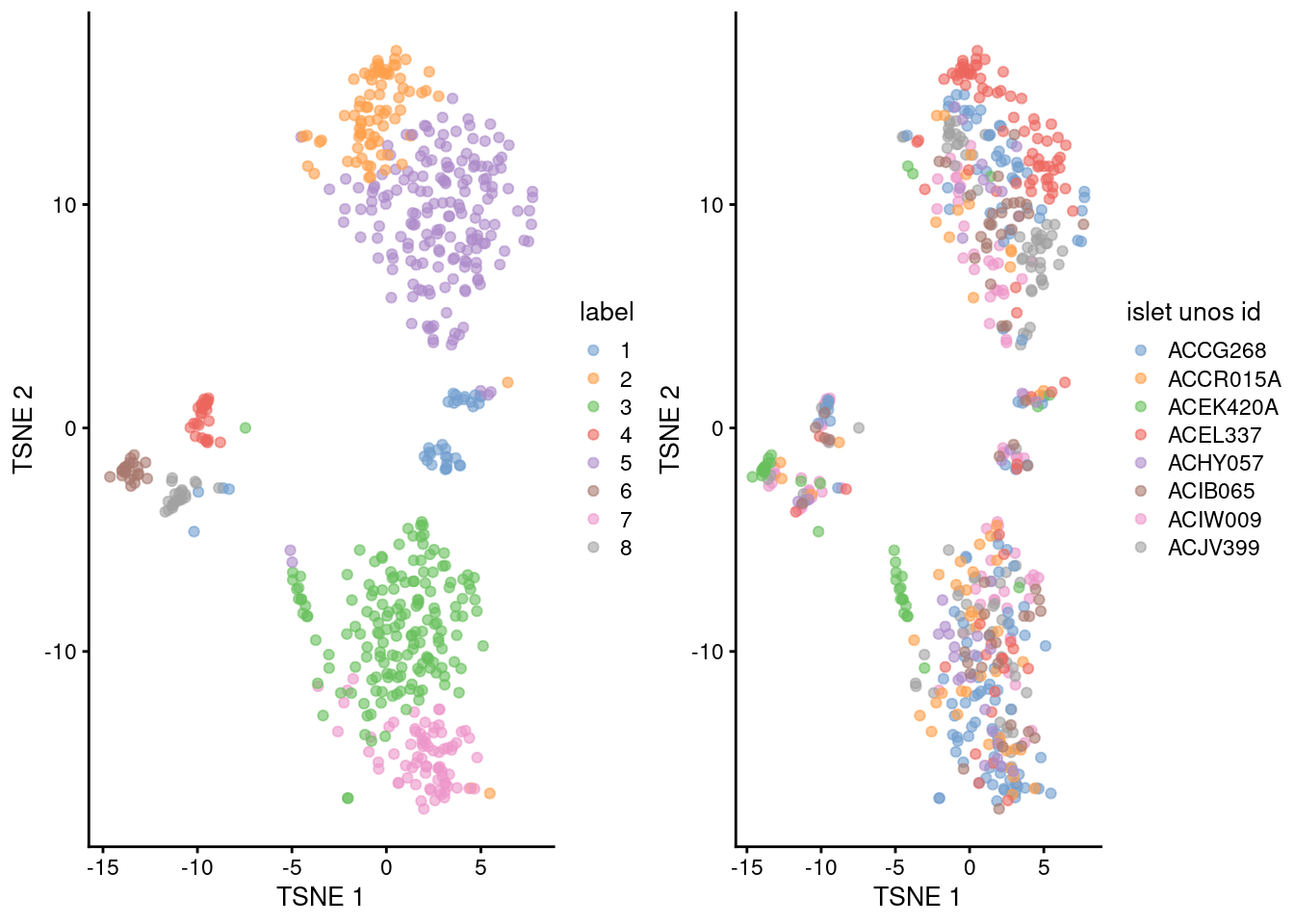
Figure 5.3: Obligatory \(t\)-SNE plots of the Lawlor pancreas dataset. Each point represents a cell that is colored by cluster (left) or batch (right).
Session Info
R version 4.3.0 RC (2023-04-13 r84269)
Platform: x86_64-pc-linux-gnu (64-bit)
Running under: Ubuntu 22.04.2 LTS

Matrix products: default
BLAS:   /home/biocbuild/bbs-3.17-bioc/R/lib/libRblas.so
LAPACK: /usr/lib/x86_64-linux-gnu/lapack/liblapack.so.3.10.0

locale:
 [1] LC_CTYPE=en_US.UTF-8       LC_NUMERIC=C
 [3] LC_TIME=en_GB              LC_COLLATE=C
 [5] LC_MONETARY=en_US.UTF-8    LC_MESSAGES=en_US.UTF-8
 [7] LC_PAPER=en_US.UTF-8       LC_NAME=C
 [9] LC_ADDRESS=C               LC_TELEPHONE=C
[11] LC_MEASUREMENT=en_US.UTF-8 LC_IDENTIFICATION=C

time zone: America/New_York
tzcode source: system (glibc)

attached base packages:
[1] stats4    stats     graphics  grDevices utils     datasets  methods
[8] base

other attached packages:
 [1] BiocSingular_1.16.0         scran_1.28.0
 [3] scater_1.28.0               ggplot2_3.4.2
 [5] scuttle_1.10.0              ensembldb_2.24.0
 [7] AnnotationFilter_1.24.0     GenomicFeatures_1.52.0
 [9] AnnotationDbi_1.62.0        AnnotationHub_3.8.0
[11] BiocFileCache_2.8.0         dbplyr_2.3.2
[13] scRNAseq_2.13.0             SingleCellExperiment_1.22.0
[15] SummarizedExperiment_1.30.0 Biobase_2.60.0
[17] GenomicRanges_1.52.0        GenomeInfoDb_1.36.0
[19] IRanges_2.34.0              S4Vectors_0.38.0
[21] BiocGenerics_0.46.0         MatrixGenerics_1.12.0
[23] matrixStats_0.63.0          BiocStyle_2.28.0
[25] rebook_1.10.0

loaded via a namespace (and not attached):
  [1] jsonlite_1.8.4                CodeDepends_0.6.5
  [3] magrittr_2.0.3                ggbeeswarm_0.7.1
  [5] farver_2.1.1                  rmarkdown_2.21
  [7] BiocIO_1.10.0                 zlibbioc_1.46.0
  [9] vctrs_0.6.2                   memoise_2.0.1
 [11] Rsamtools_2.16.0              DelayedMatrixStats_1.22.0
 [13] RCurl_1.98-1.12               htmltools_0.5.5
 [15] progress_1.2.2                curl_5.0.0
 [17] BiocNeighbors_1.18.0          sass_0.4.5
 [19] bslib_0.4.2                   cachem_1.0.7
 [21] GenomicAlignments_1.36.0      igraph_1.4.2
 [23] mime_0.12                     lifecycle_1.0.3
 [25] pkgconfig_2.0.3               rsvd_1.0.5
 [27] Matrix_1.5-4                  R6_2.5.1
 [29] fastmap_1.1.1                 GenomeInfoDbData_1.2.10
 [31] shiny_1.7.4                   digest_0.6.31
 [33] colorspace_2.1-0              dqrng_0.3.0
 [35] irlba_2.3.5.1                 ExperimentHub_2.8.0
 [37] RSQLite_2.3.1                 beachmat_2.16.0
 [39] labeling_0.4.2                filelock_1.0.2
 [41] fansi_1.0.4                   httr_1.4.5
 [43] compiler_4.3.0                bit64_4.0.5
 [45] withr_2.5.0                   BiocParallel_1.34.0
 [47] viridis_0.6.2                 DBI_1.1.3
 [49] highr_0.10                    biomaRt_2.56.0
 [51] rappdirs_0.3.3                DelayedArray_0.26.0
 [53] bluster_1.10.0                rjson_0.2.21
 [55] tools_4.3.0                   vipor_0.4.5
 [57] beeswarm_0.4.0                interactiveDisplayBase_1.38.0
 [59] httpuv_1.6.9                  glue_1.6.2
 [61] restfulr_0.0.15               promises_1.2.0.1
 [63] grid_4.3.0                    Rtsne_0.16
 [65] cluster_2.1.4                 generics_0.1.3
 [67] gtable_0.3.3                  hms_1.1.3
 [69] metapod_1.8.0                 ScaledMatrix_1.8.0
 [71] xml2_1.3.3                    utf8_1.2.3
 [73] XVector_0.40.0                ggrepel_0.9.3
 [75] BiocVersion_3.17.1            pillar_1.9.0
 [77] stringr_1.5.0                 limma_3.56.0
 [79] later_1.3.0                   dplyr_1.1.2
 [81] lattice_0.21-8                rtracklayer_1.60.0
 [83] bit_4.0.5                     tidyselect_1.2.0
 [85] locfit_1.5-9.7                Biostrings_2.68.0
 [87] knitr_1.42                    gridExtra_2.3
 [89] bookdown_0.33                 ProtGenerics_1.32.0
 [91] edgeR_3.42.0                  xfun_0.39
 [93] statmod_1.5.0                 stringi_1.7.12
 [95] lazyeval_0.2.2                yaml_2.3.7
 [97] evaluate_0.20                 codetools_0.2-19
 [99] tibble_3.2.1                  BiocManager_1.30.20
[101] graph_1.78.0                  cli_3.6.1
[103] xtable_1.8-4                  munsell_0.5.0
[105] jquerylib_0.1.4               Rcpp_1.0.10
[107] dir.expiry_1.8.0              png_0.1-8
[109] XML_3.99-0.14                 parallel_4.3.0
[111] ellipsis_0.3.2                blob_1.2.4
[113] prettyunits_1.1.1             sparseMatrixStats_1.12.0
[115] bitops_1.0-7                  viridisLite_0.4.1
[117] scales_1.2.1                  purrr_1.0.1
[119] crayon_1.5.2                  rlang_1.1.0
[121] cowplot_1.1.1                 KEGGREST_1.40.0
References
Lawlor, N., J. George, M. Bolisetty, R. Kursawe, L. Sun, V. Sivakamasundari, I. Kycia, P. Robson, and M. L. Stitzel. 2017. “Single-cell transcriptomes identify human islet cell signatures and reveal cell-type-specific expression changes in type 2 diabetes.” Genome Res. 27 (2): 208–22.