Chapter 7 Human PBMCs (10X Genomics)
7.1 Introduction
This performs an analysis of the public PBMC ID dataset generated by 10X Genomics (Zheng et al. 2017), starting from the filtered count matrix.
7.3 Quality control
Cell calling implicitly serves as a QC step to remove libraries with low total counts and number of detected genes. Thus, we will only filter on the mitochondrial proportion.
library(scater)
stats <- high.mito <- list()
for (n in names(all.sce)) {
    current <- all.sce[[n]]
    is.mito <- grep("MT", rowData(current)$Symbol_TENx)
    stats[[n]] <- perCellQCMetrics(current, subsets=list(Mito=is.mito))
    high.mito[[n]] <- isOutlier(stats[[n]]$subsets_Mito_percent, type="higher")
    all.sce[[n]] <- current[,!high.mito[[n]]]
}
qcplots <- list()
for (n in names(all.sce)) {
current <- unfiltered[[n]]
colData(current) <- cbind(colData(current), stats[[n]])
current$discard <- high.mito[[n]]
qcplots[[n]] <- plotColData(current, x="sum", y="subsets_Mito_percent",
colour_by="discard") + scale_x_log10()
}
do.call(gridExtra::grid.arrange, c(qcplots, ncol=3))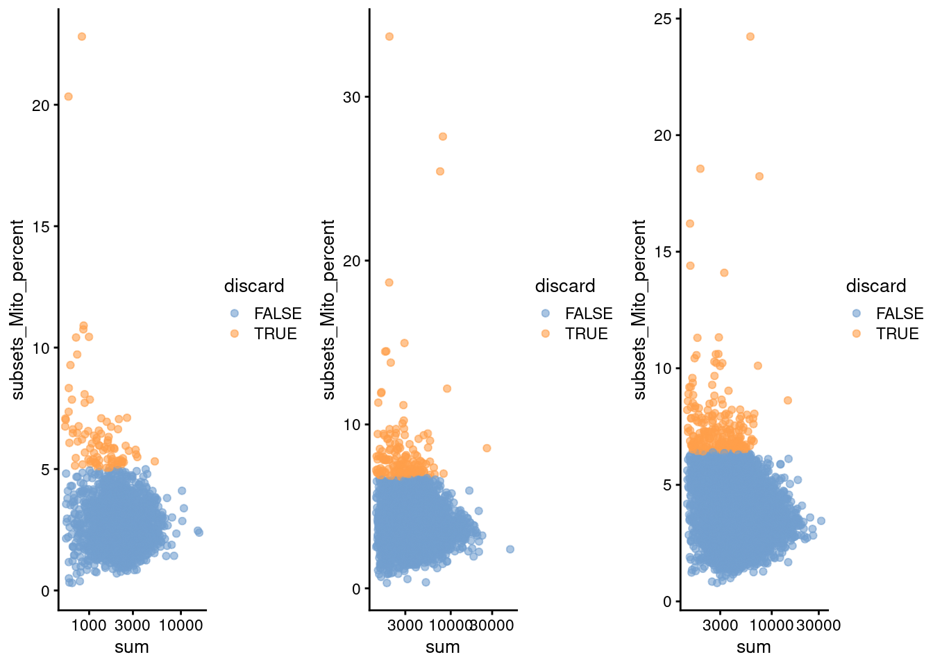
Figure 7.1: Percentage of mitochondrial reads in each cell in each of the 10X PBMC datasets, compared to the total count. Each point represents a cell and is colored according to whether that cell was discarded.
## $pbmc3k
##    Mode   FALSE    TRUE
## logical    2609      91
##
## $pbmc4k
##    Mode   FALSE    TRUE
## logical    4182     158
##
## $pbmc8k
##    Mode   FALSE    TRUE
## logical    8157     224
7.4 Normalization
We perform library size normalization, simply for convenience when dealing with file-backed matrices.
## $pbmc3k
##    Min. 1st Qu.  Median    Mean 3rd Qu.    Max.
##   0.234   0.748   0.926   1.000   1.157   6.604
##
## $pbmc4k
##    Min. 1st Qu.  Median    Mean 3rd Qu.    Max.
##   0.315   0.711   0.890   1.000   1.127  11.027
##
## $pbmc8k
##    Min. 1st Qu.  Median    Mean 3rd Qu.    Max.
##   0.296   0.704   0.877   1.000   1.118   6.794
7.5 Variance modelling
library(scran)
all.dec <- lapply(all.sce, modelGeneVar)
all.hvgs <- lapply(all.dec, getTopHVGs, prop=0.1)par(mfrow=c(1,3))
for (n in names(all.dec)) {
curdec <- all.dec[[n]]
plot(curdec$mean, curdec$total, pch=16, cex=0.5, main=n,
xlab="Mean of log-expression", ylab="Variance of log-expression")
curfit <- metadata(curdec)
curve(curfit$trend(x), col='dodgerblue', add=TRUE, lwd=2)
}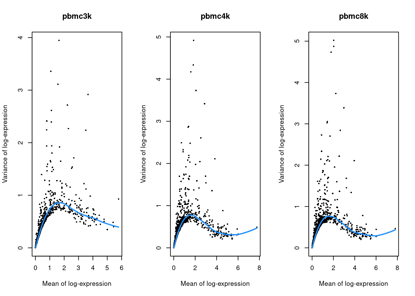
Figure 7.2: Per-gene variance as a function of the mean for the log-expression values in each PBMC dataset. Each point represents a gene (black) with the mean-variance trend (blue) fitted to the variances.
7.6 Dimensionality reduction
For various reasons, we will first analyze each PBMC dataset separately rather than merging them together. We use randomized SVD, which is more efficient for file-backed matrices.
library(BiocSingular)
set.seed(10000)
all.sce <- mapply(FUN=runPCA, x=all.sce, subset_row=all.hvgs,
    MoreArgs=list(ncomponents=25, BSPARAM=RandomParam()),
    SIMPLIFY=FALSE)

set.seed(100000)
all.sce <- lapply(all.sce, runTSNE, dimred="PCA")

set.seed(1000000)
all.sce <- lapply(all.sce, runUMAP, dimred="PCA")
7.7 Clustering
for (n in names(all.sce)) {
    g <- buildSNNGraph(all.sce[[n]], k=10, use.dimred='PCA')
    clust <- igraph::cluster_walktrap(g)$membership
    colLabels(all.sce[[n]])  <- factor(clust)
}## $pbmc3k
##
## 1 2 3 4 5 6 7 8 9 10
## 487 154 603 514 31 150 179 333 147 11
##
## $pbmc4k
##
## 1 2 3 4 5 6 7 8 9 10 11 12 13
## 497 185 569 786 373 232 44 1023 77 218 88 54 36
##
## $pbmc8k
##
## 1 2 3 4 5 6 7 8 9 10 11 12 13 14 15 16
## 1004 759 1073 1543 367 150 201 2067 59 154 244 67 76 285 20 15
## 17 18
## 64 9all.tsne <- list()
for (n in names(all.sce)) {
all.tsne[[n]] <- plotTSNE(all.sce[[n]], colour_by="label") + ggtitle(n)
}
do.call(gridExtra::grid.arrange, c(all.tsne, list(ncol=2)))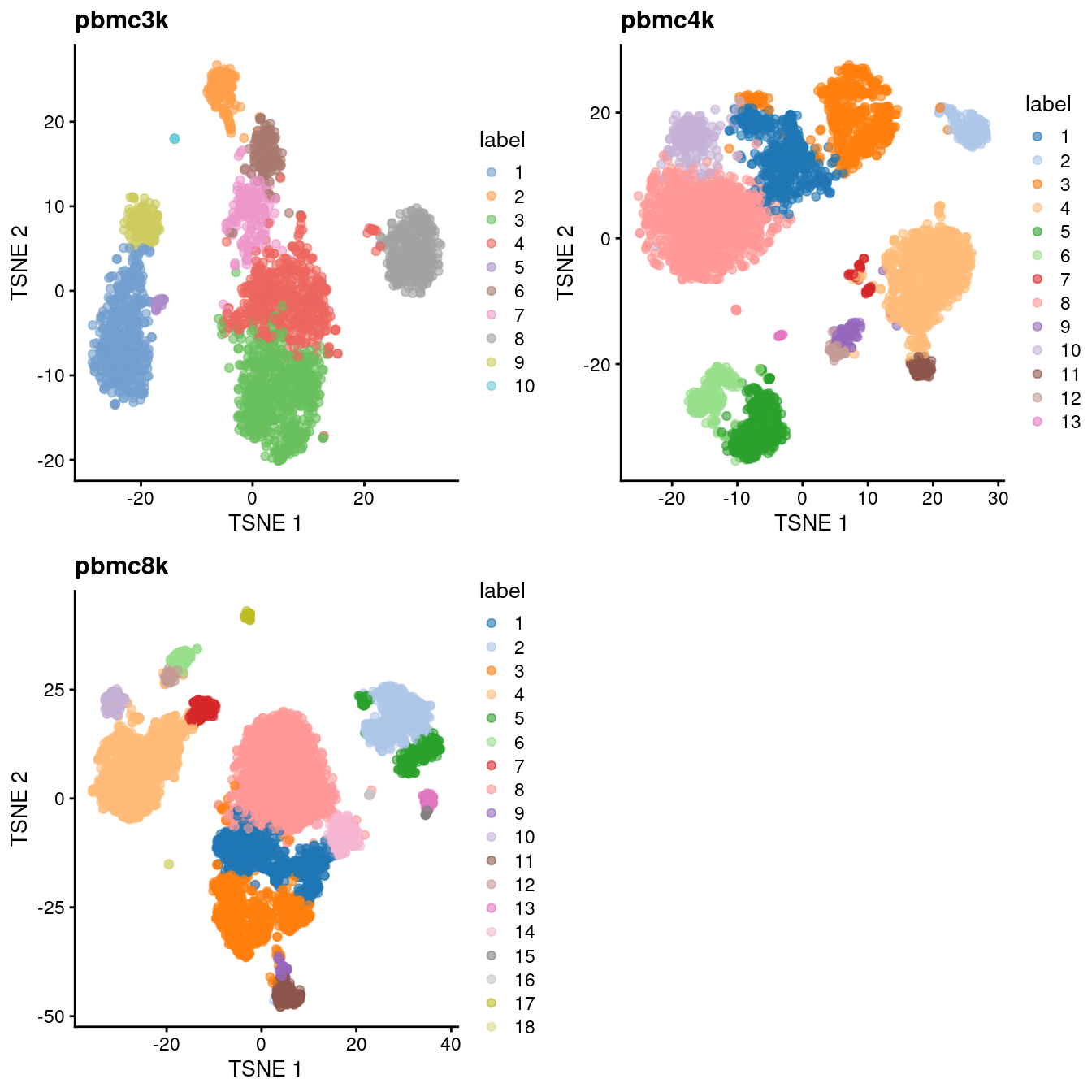
Figure 7.3: Obligatory \(t\)-SNE plots of each PBMC dataset, where each point represents a cell in the corresponding dataset and is colored according to the assigned cluster.
7.8 Data integration
With the per-dataset analyses out of the way, we will now repeat the analysis after merging together the three batches.
# Intersecting the common genes.
universe <- Reduce(intersect, lapply(all.sce, rownames))
all.sce2 <- lapply(all.sce, "[", i=universe,)
all.dec2 <- lapply(all.dec, "[", i=universe,)

# Renormalizing to adjust for differences in depth.
library(batchelor)
normed.sce <- do.call(multiBatchNorm, all.sce2)

# Identifying a set of HVGs using stats from all batches.
combined.dec <- do.call(combineVar, all.dec2)
combined.hvg <- getTopHVGs(combined.dec, n=5000)

set.seed(1000101)
merged.pbmc <- do.call(fastMNN, c(normed.sce,
    list(subset.row=combined.hvg, BSPARAM=RandomParam())))
We use the percentage of lost variance as a diagnostic measure.
##         pbmc3k    pbmc4k   pbmc8k
## [1,] 7.003e-03 3.126e-03 0.000000
## [2,] 7.137e-05 5.125e-05 0.003003
We proceed to clustering:
g <- buildSNNGraph(merged.pbmc, use.dimred="corrected")
colLabels(merged.pbmc) <- factor(igraph::cluster_louvain(g)$membership)
table(colLabels(merged.pbmc), merged.pbmc$batch)
##
## pbmc3k pbmc4k pbmc8k
## 1 523 405 826
## 2 327 588 1125
## 3 185 122 218
## 4 150 180 293
## 5 172 340 577
## 6 283 533 1002
## 7 346 638 1203
## 8 433 749 1533
## 9 17 27 111
## 10 112 387 832
## 11 34 120 204
## 12 11 54 160
## 13 12 3 9
## 14 4 36 64And visualization:
set.seed(10101010)
merged.pbmc <- runTSNE(merged.pbmc, dimred="corrected")
gridExtra::grid.arrange(
    plotTSNE(merged.pbmc, colour_by="label", text_by="label", text_colour="red"),
    plotTSNE(merged.pbmc, colour_by="batch")
)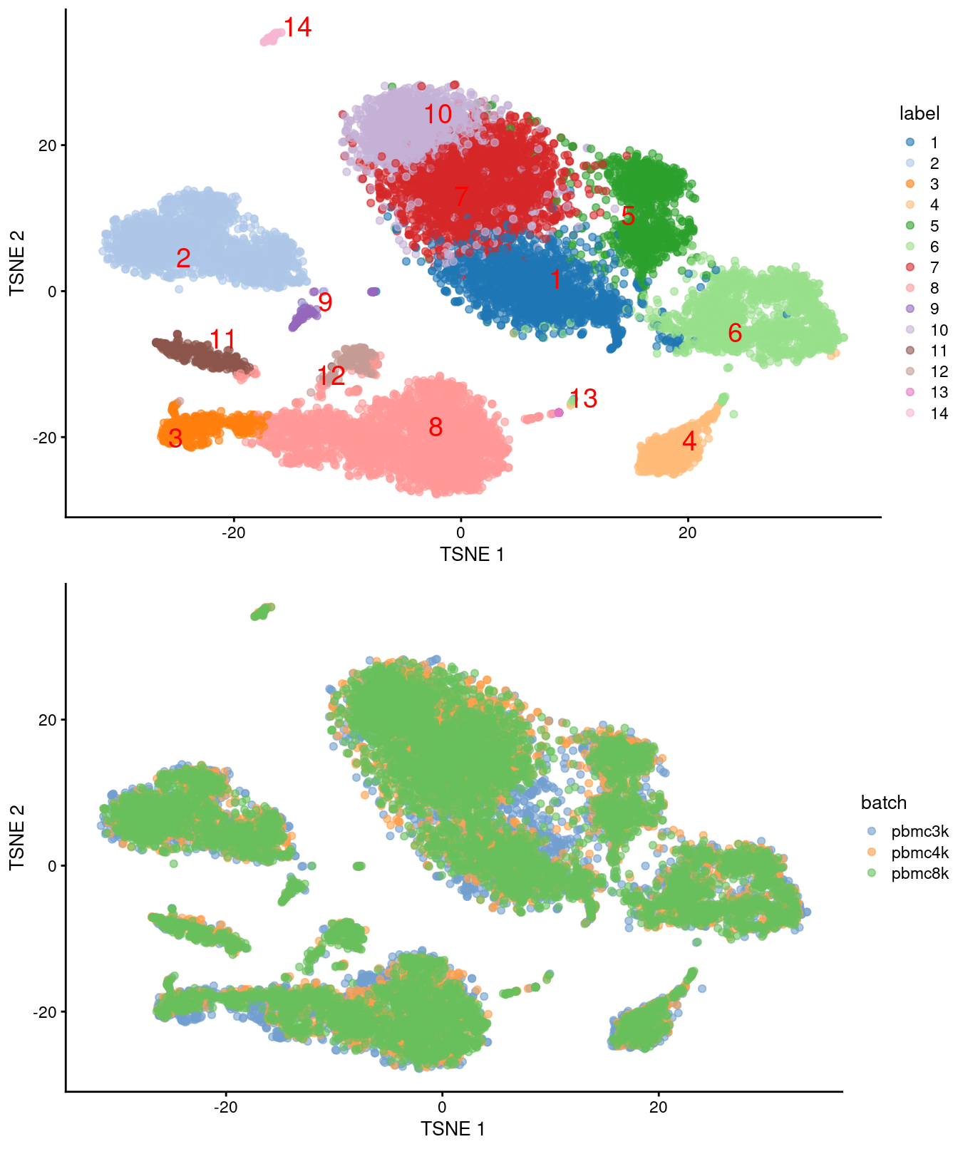
Figure 7.4: Obligatory \(t\)-SNE plots for the merged PBMC datasets, where each point represents a cell and is colored by cluster (top) or batch (bottom).
Session Info
R version 4.3.0 RC (2023-04-13 r84269)
Platform: x86_64-pc-linux-gnu (64-bit)
Running under: Ubuntu 22.04.2 LTS

Matrix products: default
BLAS:   /home/biocbuild/bbs-3.17-bioc/R/lib/libRblas.so
LAPACK: /usr/lib/x86_64-linux-gnu/lapack/liblapack.so.3.10.0

locale:
 [1] LC_CTYPE=en_US.UTF-8       LC_NUMERIC=C
 [3] LC_TIME=en_GB              LC_COLLATE=C
 [5] LC_MONETARY=en_US.UTF-8    LC_MESSAGES=en_US.UTF-8
 [7] LC_PAPER=en_US.UTF-8       LC_NAME=C
 [9] LC_ADDRESS=C               LC_TELEPHONE=C
[11] LC_MEASUREMENT=en_US.UTF-8 LC_IDENTIFICATION=C

time zone: America/New_York
tzcode source: system (glibc)

attached base packages:
[1] stats4    stats     graphics  grDevices utils     datasets  methods
[8] base

other attached packages:
 [1] batchelor_1.16.0            BiocSingular_1.16.0
 [3] scran_1.28.1                scater_1.28.0
 [5] ggplot2_3.4.2               scuttle_1.10.1
 [7] TENxPBMCData_1.18.0         HDF5Array_1.28.1
 [9] rhdf5_2.44.0                DelayedArray_0.26.2
[11] S4Arrays_1.0.4              Matrix_1.5-4
[13] SingleCellExperiment_1.22.0 SummarizedExperiment_1.30.1
[15] Biobase_2.60.0              GenomicRanges_1.52.0
[17] GenomeInfoDb_1.36.0         IRanges_2.34.0
[19] S4Vectors_0.38.1            BiocGenerics_0.46.0
[21] MatrixGenerics_1.12.0       matrixStats_0.63.0
[23] BiocStyle_2.28.0            rebook_1.10.0

loaded via a namespace (and not attached):
  [1] jsonlite_1.8.4                CodeDepends_0.6.5
  [3] magrittr_2.0.3                ggbeeswarm_0.7.2
  [5] farver_2.1.1                  rmarkdown_2.21
  [7] zlibbioc_1.46.0               vctrs_0.6.2
  [9] memoise_2.0.1                 DelayedMatrixStats_1.22.0
 [11] RCurl_1.98-1.12               htmltools_0.5.5
 [13] AnnotationHub_3.8.0           curl_5.0.0
 [15] BiocNeighbors_1.18.0          Rhdf5lib_1.22.0
 [17] sass_0.4.6                    bslib_0.4.2
 [19] cachem_1.0.8                  ResidualMatrix_1.10.0
 [21] igraph_1.4.2                  mime_0.12
 [23] lifecycle_1.0.3               pkgconfig_2.0.3
 [25] rsvd_1.0.5                    R6_2.5.1
 [27] fastmap_1.1.1                 GenomeInfoDbData_1.2.10
 [29] shiny_1.7.4                   digest_0.6.31
 [31] colorspace_2.1-0              AnnotationDbi_1.62.1
 [33] dqrng_0.3.0                   irlba_2.3.5.1
 [35] ExperimentHub_2.8.0           RSQLite_2.3.1
 [37] beachmat_2.16.0               filelock_1.0.2
 [39] labeling_0.4.2                fansi_1.0.4
 [41] httr_1.4.6                    compiler_4.3.0
 [43] bit64_4.0.5                   withr_2.5.0
 [45] BiocParallel_1.34.1           viridis_0.6.3
 [47] DBI_1.1.3                     highr_0.10
 [49] rappdirs_0.3.3                bluster_1.10.0
 [51] tools_4.3.0                   vipor_0.4.5
 [53] beeswarm_0.4.0                interactiveDisplayBase_1.38.0
 [55] httpuv_1.6.11                 glue_1.6.2
 [57] rhdf5filters_1.12.1           promises_1.2.0.1
 [59] grid_4.3.0                    Rtsne_0.16
 [61] cluster_2.1.4                 generics_0.1.3
 [63] gtable_0.3.3                  ScaledMatrix_1.8.1
 [65] metapod_1.8.0                 utf8_1.2.3
 [67] XVector_0.40.0                RcppAnnoy_0.0.20
 [69] ggrepel_0.9.3                 BiocVersion_3.17.1
 [71] pillar_1.9.0                  limma_3.56.1
 [73] later_1.3.1                   dplyr_1.1.2
 [75] BiocFileCache_2.8.0           lattice_0.21-8
 [77] FNN_1.1.3.2                   bit_4.0.5
 [79] tidyselect_1.2.0              locfit_1.5-9.7
 [81] Biostrings_2.68.1             knitr_1.42
 [83] gridExtra_2.3                 bookdown_0.34
 [85] edgeR_3.42.2                  xfun_0.39
 [87] statmod_1.5.0                 yaml_2.3.7
 [89] evaluate_0.21                 codetools_0.2-19
 [91] tibble_3.2.1                  BiocManager_1.30.20
 [93] graph_1.78.0                  cli_3.6.1
 [95] uwot_0.1.14                   xtable_1.8-4
 [97] munsell_0.5.0                 jquerylib_0.1.4
 [99] Rcpp_1.0.10                   dir.expiry_1.8.0
[101] dbplyr_2.3.2                  png_0.1-8
[103] XML_3.99-0.14                 parallel_4.3.0
[105] ellipsis_0.3.2                blob_1.2.4
[107] sparseMatrixStats_1.12.0      bitops_1.0-7
[109] viridisLite_0.4.2             scales_1.2.1
[111] purrr_1.0.1                   crayon_1.5.2
[113] rlang_1.1.1                   cowplot_1.1.1
[115] KEGGREST_1.40.0
References
Zheng, G. X., J. M. Terry, P. Belgrader, P. Ryvkin, Z. W. Bent, R. Wilson, S. B. Ziraldo, et al. 2017. “Massively parallel digital transcriptional profiling of single cells.” Nat Commun 8 (January): 14049.