Chapter 1 Quality Control
1.1 Motivation
Low-quality libraries in scRNA-seq data can arise from a variety of sources such as cell damage during dissociation or failure in library preparation (e.g., inefficient reverse transcription or PCR amplification). These usually manifest as “cells” with low total counts, few expressed genes and high mitochondrial or spike-in proportions. These low-quality libraries are problematic as they can contribute to misleading results in downstream analyses:
- They form their own distinct cluster(s), complicating interpretation of the results. This is most obviously driven by increased mitochondrial proportions or enrichment for nuclear RNAs after cell damage. In the worst case, low-quality libraries generated from different cell types can cluster together based on similarities in the damage-induced expression profiles, creating artificial intermediate states or trajectories between otherwise distinct subpopulations. Additionally, very small libraries can form their own clusters due to shifts in the mean upon transformation (Lun 2018).
- They interfere with characterization of population heterogeneity during variance estimation or principal components analysis. The first few principal components will capture differences in quality rather than biology, reducing the effectiveness of dimensionality reduction. Similarly, genes with the largest variances will be driven by differences between low- and high-quality cells. The most obvious example involves low-quality libraries with very low counts where scaling normalization inflates the apparent variance of genes that happen to have a non-zero count in those libraries.
- They contain genes that appear to be strongly “upregulated” due to aggressive scaling to normalize for small library sizes. This is most problematic for contaminating transcripts (e.g., from the ambient solution) that are present in all libraries at low but constant levels. Increased scaling in low-quality libraries transforms small counts for these transcripts in large normalized expression values, resulting in apparent upregulation compared to other cells. This can be misleading as the affected genes are often biologically sensible but are actually expressed in another subpopulation.
To avoid - or at least mitigate - these problems, we need to remove the problematic cells at the start of the analysis. This step is commonly referred to as quality control (QC) on the cells. (We will use “library” and “cell” rather interchangeably here, though the distinction will become important when dealing with droplet-based data.) We demonstrate using a small scRNA-seq dataset from Lun et al. (2017), which is provided with no prior QC so that we can apply our own procedures.
## class: SingleCellExperiment
## dim: 46604 192
## metadata(0):
## assays(1): counts
## rownames(46604): ENSMUSG00000102693 ENSMUSG00000064842 ...
##   ENSMUSG00000095742 CBFB-MYH11-mcherry
## rowData names(1): Length
## colnames(192): SLX-9555.N701_S502.C89V9ANXX.s_1.r_1
##   SLX-9555.N701_S503.C89V9ANXX.s_1.r_1 ...
##   SLX-11312.N712_S508.H5H5YBBXX.s_8.r_1
##   SLX-11312.N712_S517.H5H5YBBXX.s_8.r_1
## colData names(9): Source Name cell line ... spike-in addition block
## reducedDimNames(0):
## mainExpName: endogenous
## altExpNames(2): ERCC SIRV
1.2 Common choices of QC metrics
We use several common QC metrics to identify low-quality cells based on their expression profiles. These metrics are described below in terms of reads for SMART-seq2 data, but the same definitions apply to UMI data generated by other technologies like MARS-seq and droplet-based protocols.
- The library size is defined as the total sum of counts across all relevant features for each cell. Here, we will consider the relevant features to be the endogenous genes. Cells with small library sizes are of low quality as the RNA has been lost at some point during library preparation, either due to cell lysis or inefficient cDNA capture and amplification.
- The number of expressed features in each cell is defined as the number of endogenous genes with non-zero counts for that cell. Any cell with very few expressed genes is likely to be of poor quality as the diverse transcript population has not been successfully captured.
- The proportion of reads mapped to spike-in transcripts is calculated relative to the total count across all features (including spike-ins) for each cell. As the same amount of spike-in RNA should have been added to each cell, any enrichment in spike-in counts is symptomatic of loss of endogenous RNA. Thus, high proportions are indicative of poor-quality cells where endogenous RNA has been lost due to, e.g., partial cell lysis or RNA degradation during dissociation.
- In the absence of spike-in transcripts, the proportion of reads mapped to genes in the mitochondrial genome can be used. High proportions are indicative of poor-quality cells (Islam et al. 2014; Ilicic et al. 2016), presumably because of loss of cytoplasmic RNA from perforated cells. The reasoning is that, in the presence of modest damage, the holes in the cell membrane permit efflux of individual transcript molecules but are too small to allow mitochondria to escape, leading to a relative enrichment of mitochondrial transcripts. For single-nuclei RNA-seq experiments, high proportions are also useful as they can mark cells where the cytoplasm has not been successfully stripped.
For each cell, we calculate these QC metrics using the perCellQCMetrics() function from the scater package (McCarthy et al. 2017).
The sum column contains the total count for each cell and the detected column contains the number of detected genes.
The subsets_Mito_percent column contains the percentage of reads mapped to mitochondrial transcripts.
Finally, the altexps_ERCC_percent column contains the percentage of reads mapped to ERCC transcripts.
# Identifying the mitochondrial transcripts in our SingleCellExperiment.
location <- rowRanges(sce.416b)
is.mito <- any(seqnames(location)=="MT")

library(scuttle)
df <- perCellQCMetrics(sce.416b, subsets=list(Mito=is.mito))
summary(df$sum)
## Min. 1st Qu. Median Mean 3rd Qu. Max.
## 27084 856350 1111252 1165865 1328301 4398883## Min. 1st Qu. Median Mean 3rd Qu. Max.
## 5609 7502 8341 8397 9208 11380## Min. 1st Qu. Median Mean 3rd Qu. Max.
## 4.59 7.29 8.14 8.15 9.04 15.62## Min. 1st Qu. Median Mean 3rd Qu. Max.
## 2.24 4.29 6.03 6.41 8.13 19.43Alternatively, users may prefer to use the addPerCellQC() function.
This computes and appends the per-cell QC statistics to the colData of the SingleCellExperiment object,
allowing us to retain all relevant information in a single object for later manipulation.
##  [1] "Source Name"              "cell line"
##  [3] "cell type"                "single cell well quality"
##  [5] "genotype"                 "phenotype"
##  [7] "strain"                   "spike-in addition"
##  [9] "block"                    "sum"
## [11] "detected"                 "subsets_Mito_sum"
## [13] "subsets_Mito_detected"    "subsets_Mito_percent"
## [15] "altexps_ERCC_sum"         "altexps_ERCC_detected"
## [17] "altexps_ERCC_percent"     "altexps_SIRV_sum"
## [19] "altexps_SIRV_detected"    "altexps_SIRV_percent"
## [21] "total"
A key assumption here is that the QC metrics are independent of the biological state of each cell. Poor values (e.g., low library sizes, high mitochondrial proportions) are presumed to be driven by technical factors rather than biological processes, meaning that the subsequent removal of cells will not misrepresent the biology in downstream analyses. Major violations of this assumption would potentially result in the loss of cell types that have, say, systematically low RNA content or high numbers of mitochondria. We can check for such violations using diagnostic plots described in Section 1.4 and Advanced Section 1.5.
1.3 Identifying low-quality cells
1.3.1 With fixed thresholds
The simplest approach to identifying low-quality cells involves applying fixed thresholds to the QC metrics. For example, we might consider cells to be low quality if they have library sizes below 100,000 reads; express fewer than 5,000 genes; have spike-in proportions above 10%; or have mitochondrial proportions above 10%.
qc.lib <- df$sum < 1e5
qc.nexprs <- df$detected < 5e3
qc.spike <- df$altexps_ERCC_percent > 10
qc.mito <- df$subsets_Mito_percent > 10
discard <- qc.lib | qc.nexprs | qc.spike | qc.mito

# Summarize the number of cells removed for each reason.
DataFrame(LibSize=sum(qc.lib), NExprs=sum(qc.nexprs),
    SpikeProp=sum(qc.spike), MitoProp=sum(qc.mito), Total=sum(discard))
## DataFrame with 1 row and 5 columns
## LibSize NExprs SpikeProp MitoProp Total
## <integer> <integer> <integer> <integer> <integer>
## 1 3 0 19 14 33While simple, this strategy requires considerable experience to determine appropriate thresholds for each experimental protocol and biological system. Thresholds for read count-based data are not applicable for UMI-based data, and vice versa. Differences in mitochondrial activity or total RNA content require constant adjustment of the mitochondrial and spike-in thresholds, respectively, for different biological systems. Indeed, even with the same protocol and system, the appropriate threshold can vary from run to run due to the vagaries of cDNA capture efficiency and sequencing depth per cell.
1.3.2 With adaptive thresholds
Here, we assume that most of the dataset consists of high-quality cells.
We then identify cells that are outliers for the various QC metrics, based on the median absolute deviation (MAD) from the median value of each metric across all cells.
By default, we consider a value to be an outlier if it is more than 3 MADs from the median in the “problematic” direction.
This is loosely motivated by the fact that such a filter will retain 99% of non-outlier values that follow a normal distribution.
We demonstrate by using the perCellQCFilters() function on the QC metrics from the 416B dataset.
reasons <- perCellQCFilters(df,
    sub.fields=c("subsets_Mito_percent", "altexps_ERCC_percent"))
colSums(as.matrix(reasons))
## low_lib_size low_n_features high_subsets_Mito_percent
## 4 0 2
## high_altexps_ERCC_percent discard
## 1 6This function will identify cells with log-transformed library sizes that are more than 3 MADs below the median.
A log-transformation is used to improve resolution at small values when type="lower"
and to avoid negative thresholds that would be meaningless for a non-negative metric.
Furthermore, it is not uncommon for the distribution of library sizes to exhibit a heavy right tail;
the log-transformation avoids inflation of the MAD in a manner that might compromise outlier detection on the left tail.
(More generally, it makes the distribution seem more normal to justify the 99% rationale mentioned above.)
The function will also do the same for the log-transformed number of expressed genes.
perCellQCFilters() will also identify outliers for the proportion-based metrics specified in the sub.fields= arguments.
These distributions frequently exhibit a heavy right tail, but unlike the two previous metrics, it is the right tail itself that contains the putative low-quality cells.
Thus, we do not perform any transformation to shrink the tail - rather, our hope is that the cells in the tail are identified as large outliers.
(While it is theoretically possible to obtain a meaningless threshold above 100%, this is rare enough to not be of practical concern.)
A cell that is an outlier for any of these metrics is considered to be of low quality and discarded.
This is captured in the discard column, which can be used for later filtering (Section 1.5).
##    Mode   FALSE    TRUE
## logical     186       6
We can also extract the exact filter thresholds from the attributes of each of the logical vectors. This may be useful for checking whether the automatically selected thresholds are appropriate.
##  lower higher
## 434083 Inf## lower higher
## 5231 InfWith this strategy, the thresholds adapt to both the location and spread of the distribution of values for a given metric. This allows the QC procedure to adjust to changes in sequencing depth, cDNA capture efficiency, mitochondrial content, etc. without requiring any user intervention or prior experience. However, the underlying assumption of a high-quality majority may not always be appropriate, which is discussed in more detail in Advanced Section 1.3.
1.3.3 Other approaches
Another strategy is to identify outliers in high-dimensional space based on the QC metrics for each cell.
We use methods from robustbase to quantify the “outlyingness” of each cells based on their QC metrics, and then use isOutlier() to identify low-quality cells that exhibit unusually high levels of outlyingness.
stats <- cbind(log10(df$sum), log10(df$detected),
    df$subsets_Mito_percent, df$altexps_ERCC_percent)

library(robustbase)
outlying <- adjOutlyingness(stats, only.outlyingness = TRUE)
multi.outlier <- isOutlier(outlying, type = "higher")
summary(multi.outlier)
## Mode FALSE TRUE
## logical 182 10This and related approaches like PCA-based outlier detection and support vector machines can provide more power to distinguish low-quality cells from high-quality counterparts (Ilicic et al. 2016) as they can exploit patterns across many QC metrics. However, this comes at some cost to interpretability, as the reason for removing a given cell may not always be obvious.
For completeness, we note that outliers can also be identified from the gene expression profiles, rather than QC metrics. We consider this to be a risky strategy as it can remove high-quality cells in rare populations.
1.4 Checking diagnostic plots
It is good practice to inspect the distributions of QC metrics (Figure 1.1) to identify possible problems. In the most ideal case, we would see normal distributions that would justify the 3 MAD threshold used in outlier detection. A large proportion of cells in another mode suggests that the QC metrics might be correlated with some biological state, potentially leading to the loss of distinct cell types during filtering; or that there were inconsistencies with library preparation for a subset of cells, a not-uncommon phenomenon in plate-based protocols.
colData(sce.416b) <- cbind(colData(sce.416b), df)
sce.416b$block <- factor(sce.416b$block)
sce.416b$phenotype <- ifelse(grepl("induced", sce.416b$phenotype),
    "induced", "wild type")
sce.416b$discard <- reasons$discard

library(scater)
gridExtra::grid.arrange(
    plotColData(sce.416b, x="block", y="sum", colour_by="discard",
        other_fields="phenotype") + facet_wrap(~phenotype) +
        scale_y_log10() + ggtitle("Total count"),
    plotColData(sce.416b, x="block", y="detected", colour_by="discard",
        other_fields="phenotype") + facet_wrap(~phenotype) +
        scale_y_log10() + ggtitle("Detected features"),
    plotColData(sce.416b, x="block", y="subsets_Mito_percent",
        colour_by="discard", other_fields="phenotype") +
        facet_wrap(~phenotype) + ggtitle("Mito percent"),
    plotColData(sce.416b, x="block", y="altexps_ERCC_percent",
        colour_by="discard", other_fields="phenotype") +
        facet_wrap(~phenotype) + ggtitle("ERCC percent"),
    ncol=1
)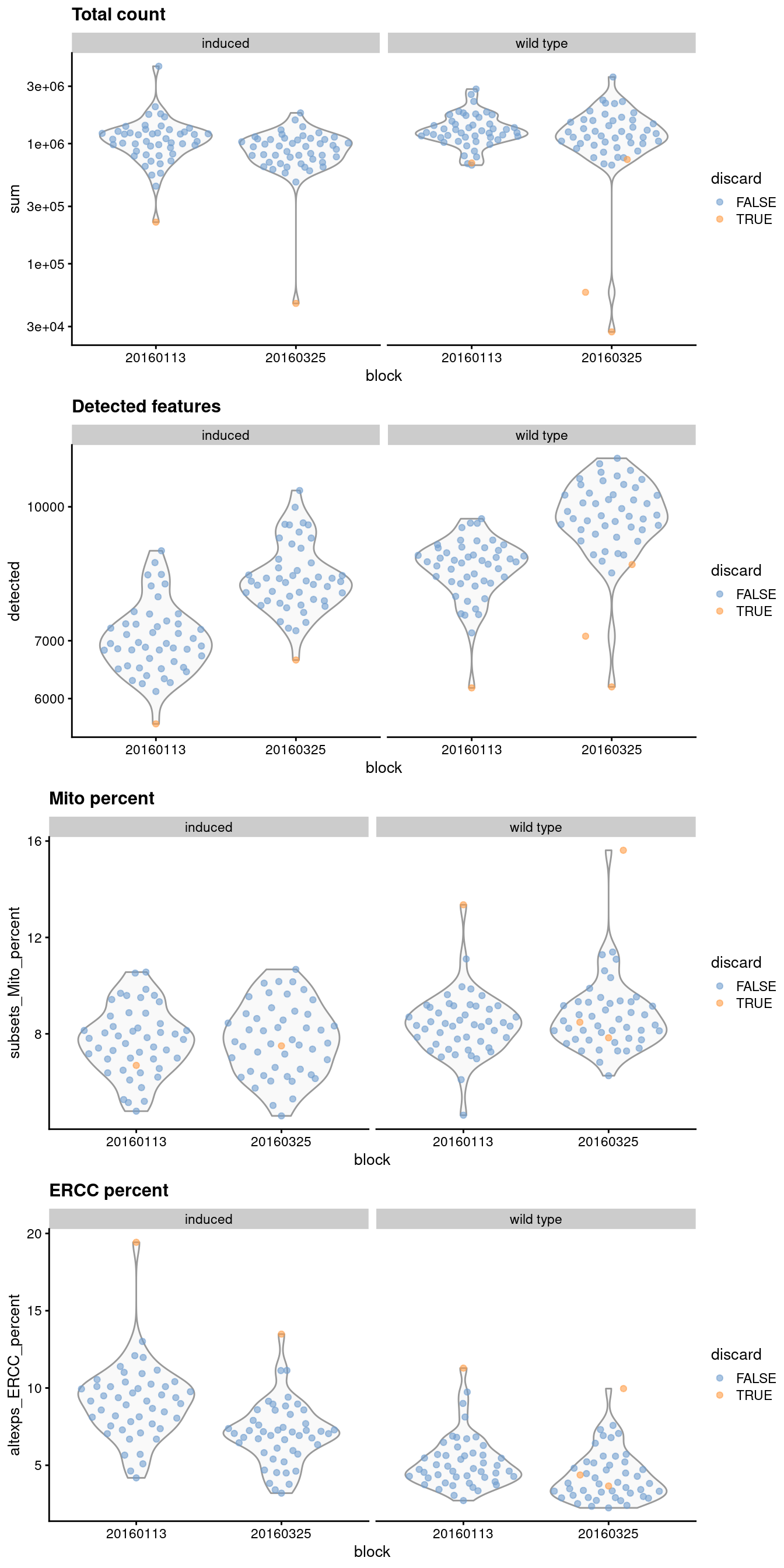
Figure 1.1: Distribution of QC metrics for each batch and phenotype in the 416B dataset. Each point represents a cell and is colored according to whether it was discarded, respectively.
Another useful diagnostic involves plotting the proportion of mitochondrial counts against some of the other QC metrics. The aim is to confirm that there are no cells with both large total counts and large mitochondrial counts, to ensure that we are not inadvertently removing high-quality cells that happen to be highly metabolically active (e.g., hepatocytes). We demonstrate using data from a larger experiment involving the mouse brain (Zeisel et al. 2015); in this case, we do not observe any points in the top-right corner in Figure 1.2 that might potentially correspond to metabolically active, undamaged cells.
#--- loading ---#
library(scRNAseq)
sce.zeisel <- ZeiselBrainData()

library(scater)
sce.zeisel <- aggregateAcrossFeatures(sce.zeisel,
    id=sub("_loc[0-9]+$", "", rownames(sce.zeisel)))

#--- gene-annotation ---#
library(org.Mm.eg.db)
rowData(sce.zeisel)$Ensembl <- mapIds(org.Mm.eg.db,
    keys=rownames(sce.zeisel), keytype="SYMBOL", column="ENSEMBL")
sce.zeisel <- addPerCellQC(sce.zeisel,
subsets=list(Mt=rowData(sce.zeisel)$featureType=="mito"))
qc <- quickPerCellQC(colData(sce.zeisel),
sub.fields=c("altexps_ERCC_percent", "subsets_Mt_percent"))
sce.zeisel$discard <- qc$discard
plotColData(sce.zeisel, x="sum", y="subsets_Mt_percent", colour_by="discard")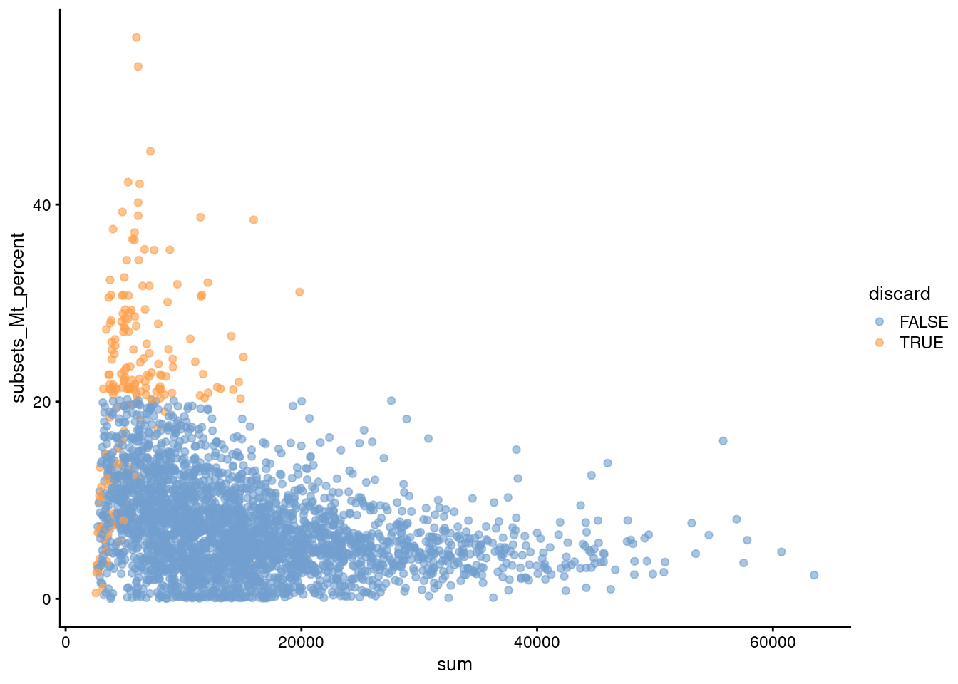
Figure 1.2: Percentage of UMIs assigned to mitochondrial transcripts in the Zeisel brain dataset, plotted against the total number of UMIs (top). Each point represents a cell and is colored according to whether it was considered low-quality and discarded.
Comparison of the ERCC and mitochondrial percentages can also be informative (Figure 1.3). Low-quality cells with small mitochondrial percentages, large spike-in percentages and small library sizes are likely to be stripped nuclei, i.e., they have been so extensively damaged that they have lost all cytoplasmic content. On the other hand, cells with high mitochondrial percentages and low ERCC percentages may represent undamaged cells that are metabolically active. This interpretation also applies for single-nuclei studies but with a switch of focus: the stripped nuclei become the libraries of interest while the undamaged cells are considered to be low quality.
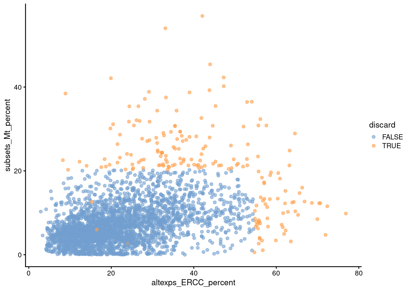
Figure 1.3: Percentage of UMIs assigned to mitochondrial transcripts in the Zeisel brain dataset, plotted against the percentage of UMIs assigned to spike-in transcripts (bottom). Each point represents a cell and is colored according to whether it was considered low-quality and discarded.
We see that all of these metrics exhibit weak correlations to each other, presumably a manifestation of a common underlying effect of cell damage. The weakness of the correlations motivates the use of several metrics to capture different aspects of technical quality. Of course, the flipside is that these metrics may also represent different aspects of biology, increasing the risk of inadvertently discarding entire cell types.
1.5 Removing low-quality cells
Once low-quality cells have been identified, we can choose to either remove them or mark them.
Removal is the most straightforward option and is achieved by subsetting the SingleCellExperiment by column.
In this case, we use the low-quality calls from Section 1.3.2 to generate a subsetted SingleCellExperiment that we would use for downstream analyses.
The other option is to simply mark the low-quality cells as such and retain them in the downstream analysis. The aim here is to allow clusters of low-quality cells to form, and then to identify and ignore such clusters during interpretation of the results. This approach avoids discarding cell types that have poor values for the QC metrics, deferring the decision on whether a cluster of such cells represents a genuine biological state.
The downside is that it shifts the burden of QC to the manual interpretation of the clusters, which is already a major bottleneck in scRNA-seq data analysis (Chapters 5, 6 and 7). Indeed, if we do not trust the QC metrics, we would have to distinguish between genuine cell types and low-quality cells based only on marker genes, and this is not always easy due to the tendency of the latter to “express” interesting genes (Section 1.1). Retention of low-quality cells also compromises the accuracy of the variance modelling, requiring, e.g., use of more PCs to offset the fact that the early PCs are driven by differences between low-quality and other cells.
For routine analyses, we suggest performing removal by default to avoid complications from low-quality cells. This allows most of the population structure to be characterized with no - or, at least, fewer - concerns about its validity. Once the initial analysis is done, and if there are any concerns about discarded cell types (Advanced Section 1.5), a more thorough re-analysis can be performed where the low-quality cells are only marked. This recovers cell types with low RNA content, high mitochondrial proportions, etc. that only need to be interpreted insofar as they “fill the gaps” in the initial analysis.
Session Info
R version 4.2.2 (2022-10-31)
Platform: x86_64-pc-linux-gnu (64-bit)
Running under: Ubuntu 20.04.5 LTS

Matrix products: default
BLAS:   /home/biocbuild/bbs-3.16-bioc/R/lib/libRblas.so
LAPACK: /home/biocbuild/bbs-3.16-bioc/R/lib/libRlapack.so

locale:
 [1] LC_CTYPE=en_US.UTF-8       LC_NUMERIC=C
 [3] LC_TIME=en_GB              LC_COLLATE=C
 [5] LC_MONETARY=en_US.UTF-8    LC_MESSAGES=en_US.UTF-8
 [7] LC_PAPER=en_US.UTF-8       LC_NAME=C
 [9] LC_ADDRESS=C               LC_TELEPHONE=C
[11] LC_MEASUREMENT=en_US.UTF-8 LC_IDENTIFICATION=C

attached base packages:
[1] stats4    stats     graphics  grDevices utils     datasets  methods
[8] base

other attached packages:
 [1] scater_1.26.1               ggplot2_3.4.1
 [3] robustbase_0.95-0           scuttle_1.8.4
 [5] SingleCellExperiment_1.20.0 SummarizedExperiment_1.28.0
 [7] Biobase_2.58.0              GenomicRanges_1.50.2
 [9] GenomeInfoDb_1.34.9         IRanges_2.32.0
[11] S4Vectors_0.36.1            BiocGenerics_0.44.0
[13] MatrixGenerics_1.10.0       matrixStats_0.63.0
[15] BiocStyle_2.26.0            rebook_1.8.0

loaded via a namespace (and not attached):
 [1] viridis_0.6.2             sass_0.4.5
 [3] BiocSingular_1.14.0       viridisLite_0.4.1
 [5] jsonlite_1.8.4            DelayedMatrixStats_1.20.0
 [7] bslib_0.4.2               highr_0.10
 [9] BiocManager_1.30.19       vipor_0.4.5
[11] GenomeInfoDbData_1.2.9    ggrepel_0.9.3
[13] yaml_2.3.7                pillar_1.8.1
[15] lattice_0.20-45           glue_1.6.2
[17] beachmat_2.14.0           digest_0.6.31
[19] XVector_0.38.0            colorspace_2.1-0
[21] cowplot_1.1.1             htmltools_0.5.4
[23] Matrix_1.5-3              XML_3.99-0.13
[25] pkgconfig_2.0.3           dir.expiry_1.6.0
[27] bookdown_0.32             zlibbioc_1.44.0
[29] scales_1.2.1              ScaledMatrix_1.6.0
[31] BiocParallel_1.32.5       tibble_3.1.8
[33] farver_2.1.1              generics_0.1.3
[35] cachem_1.0.6              withr_2.5.0
[37] cli_3.6.0                 magrittr_2.0.3
[39] CodeDepends_0.6.5         evaluate_0.20
[41] fansi_1.0.4               beeswarm_0.4.0
[43] graph_1.76.0              tools_4.2.2
[45] lifecycle_1.0.3           munsell_0.5.0
[47] DelayedArray_0.24.0       irlba_2.3.5.1
[49] compiler_4.2.2            jquerylib_0.1.4
[51] rsvd_1.0.5                rlang_1.0.6
[53] grid_4.2.2                RCurl_1.98-1.10
[55] BiocNeighbors_1.16.0      rappdirs_0.3.3
[57] labeling_0.4.2            bitops_1.0-7
[59] rmarkdown_2.20            gtable_0.3.1
[61] codetools_0.2-19          R6_2.5.1
[63] gridExtra_2.3             knitr_1.42
[65] dplyr_1.1.0               fastmap_1.1.0
[67] utf8_1.2.3                filelock_1.0.2
[69] ggbeeswarm_0.7.1          parallel_4.2.2
[71] Rcpp_1.0.10               vctrs_0.5.2
[73] DEoptimR_1.0-11           tidyselect_1.2.0
[75] xfun_0.37                 sparseMatrixStats_1.10.0
References
Ilicic, T., J. K. Kim, A. A. Kołodziejczyk, F. O. Bagger, D. J. McCarthy, J. C. Marioni, and S. A. Teichmann. 2016. “Classification of low quality cells from single-cell RNA-seq data.” Genome Biol. 17 (1): 29.
Islam, S., A. Zeisel, S. Joost, G. La Manno, P. Zajac, M. Kasper, P. Lonnerberg, and S. Linnarsson. 2014. “Quantitative single-cell RNA-seq with unique molecular identifiers.” Nat. Methods 11 (2): 163–66.
Lun, A. 2018. “Overcoming Systematic Errors Caused by Log-Transformation of Normalized Single-Cell Rna Sequencing Data.” bioRxiv.
Lun, A. T. L., F. J. Calero-Nieto, L. Haim-Vilmovsky, B. Gottgens, and J. C. Marioni. 2017. “Assessing the reliability of spike-in normalization for analyses of single-cell RNA sequencing data.” Genome Res. 27 (11): 1795–1806.
McCarthy, D. J., K. R. Campbell, A. T. Lun, and Q. F. Wills. 2017. “Scater: pre-processing, quality control, normalization and visualization of single-cell RNA-seq data in R.” Bioinformatics 33 (8): 1179–86.
Zeisel, A., A. B. Munoz-Manchado, S. Codeluppi, P. Lonnerberg, G. La Manno, A. Jureus, S. Marques, et al. 2015. “Brain structure. Cell types in the mouse cortex and hippocampus revealed by single-cell RNA-seq.” Science 347 (6226): 1138–42.