Chapter 3 Using the corrected values
3.1 Background
The greatest value of batch correction lies in facilitating cell-based analysis of population heterogeneity in a consistent manner across batches. Cluster 1 in batch A is the same as cluster 1 in batch B when the clustering is performed on the merged data. There is no need to identify mappings between separate clusterings, which might not even be possible when the clusters are not well-separated. By generating a single set of clusters for all batches, rather than requiring separate examination of each batch’s clusters, we avoid repeatedly paying the cost of manual interpretation. Another benefit is that the available number of cells is increased when all batches are combined, which allows for greater resolution of population structure in downstream analyses.
We previously demonstrated the application of clustering methods to the batch-corrected data, but the same principles apply for other analyses like trajectory reconstruction.
In general, cell-based analyses are safe to apply on corrected data; indeed, the whole purpose of the correction is to place all cells in the same coordinate space.
However, the same cannot be easily said for gene-based procedures like DE analyses or marker gene detection.
An arbitrary correction algorithm is not obliged to preserve relative differences in per-gene expression when attempting to align multiple batches.
For example, cosine normalization in fastMNN() shrinks the magnitude of the expression values so that the computed log-fold changes have no obvious interpretation.
This chapter will elaborate on some of the problems with using corrected values for gene-based analyses. We consider both within-batch analyses like marker detection as well as between-batch comparisons.
3.2 For within-batch comparisons
Correction is not guaranteed to preserve relative differences between cells in the same batch. This complicates the intepretation of corrected values for within-batch analyses such as marker detection. To demonstrate, consider the two pancreas datasets from Grun et al. (2016) and Muraro et al. (2016).
#--- loading ---#
library(scRNAseq)
sce.muraro <- MuraroPancreasData()

#--- gene-annotation ---#
library(AnnotationHub)
edb <- AnnotationHub()[["AH73881"]]
gene.symb <- sub("__chr.*$", "", rownames(sce.muraro))
gene.ids <- mapIds(edb, keys=gene.symb,
    keytype="SYMBOL", column="GENEID")

# Removing duplicated genes or genes without Ensembl IDs.
keep <- !is.na(gene.ids) & !duplicated(gene.ids)
sce.muraro <- sce.muraro[keep,]
rownames(sce.muraro) <- gene.ids[keep]

#--- quality-control ---#
library(scater)
stats <- perCellQCMetrics(sce.muraro)
qc <- quickPerCellQC(stats, percent_subsets="altexps_ERCC_percent",
    batch=sce.muraro$donor, subset=sce.muraro$donor!="D28")
sce.muraro <- sce.muraro[,!qc$discard]

#--- normalization ---#
library(scran)
set.seed(1000)
clusters <- quickCluster(sce.muraro)
sce.muraro <- computeSumFactors(sce.muraro, clusters=clusters)
sce.muraro <- logNormCounts(sce.muraro)

#--- variance-modelling ---#
block <- paste0(sce.muraro$plate, "_", sce.muraro$donor)
dec.muraro <- modelGeneVarWithSpikes(sce.muraro, "ERCC", block=block)
top.muraro <- getTopHVGs(dec.muraro, prop=0.1)## class: SingleCellExperiment
## dim: 16940 2299
## metadata(0):
## assays(2): counts logcounts
## rownames(16940): ENSG00000268895 ENSG00000121410 ... ENSG00000159840
## ENSG00000074755
## rowData names(2): symbol chr
## colnames(2299): D28-1_1 D28-1_2 ... D30-8_93 D30-8_94
## colData names(4): label donor plate sizeFactor
## reducedDimNames(0):
## mainExpName: endogenous
## altExpNames(1): ERCC#--- loading ---#
library(scRNAseq)
sce.grun <- GrunPancreasData()
#--- gene-annotation ---#
library(org.Hs.eg.db)
gene.ids <- mapIds(org.Hs.eg.db, keys=rowData(sce.grun)$symbol,
keytype="SYMBOL", column="ENSEMBL")
keep <- !is.na(gene.ids) & !duplicated(gene.ids)
sce.grun <- sce.grun[keep,]
rownames(sce.grun) <- gene.ids[keep]
#--- quality-control ---#
library(scater)
stats <- perCellQCMetrics(sce.grun)
qc <- quickPerCellQC(stats, percent_subsets="altexps_ERCC_percent",
batch=sce.grun$donor,
subset=sce.grun$donor %in% c("D17", "D7", "D2"))
sce.grun <- sce.grun[,!qc$discard]
#--- normalization ---#
library(scran)
set.seed(1000) # for irlba.
clusters <- quickCluster(sce.grun)
sce.grun <- computeSumFactors(sce.grun, clusters=clusters)
sce.grun <- logNormCounts(sce.grun)
#--- variance-modelling ---#
block <- paste0(sce.grun$sample, "_", sce.grun$donor)
dec.grun <- modelGeneVarWithSpikes(sce.grun, spikes="ERCC", block=block)
top.grun <- getTopHVGs(dec.grun, prop=0.1)# Applying cell type labels for downstream interpretation.
library(SingleR)
training <- sce.muraro[,!is.na(sce.muraro$label)]
assignments <- SingleR(sce.grun, training, labels=training$label)
sce.grun$label <- assignments$labels
sce.grun## class: SingleCellExperiment
## dim: 17331 1063
## metadata(0):
## assays(2): counts logcounts
## rownames(17331): ENSG00000268895 ENSG00000121410 ... ENSG00000074755
## ENSG00000036549
## rowData names(2): symbol chr
## colnames(1063): D2ex_1 D2ex_2 ... D17TGFB_94 D17TGFB_95
## colData names(4): donor sample sizeFactor label
## reducedDimNames(0):
## mainExpName: endogenous
## altExpNames(1): ERCCIf we look at the expression of the INS-IGF2 transcript, we can see that there is a major difference between the two batches (Figure 3.1). This is most likely due to some difference in read mapping stringency between the two studies, but the exact cause is irrelevant to this example.
library(scater)
gridExtra::grid.arrange(
    plotExpression(sce.grun, x="label", features="ENSG00000129965") + ggtitle("Grun"),
    plotExpression(sce.muraro, x="label", features="ENSG00000129965") + ggtitle("Muraro")
)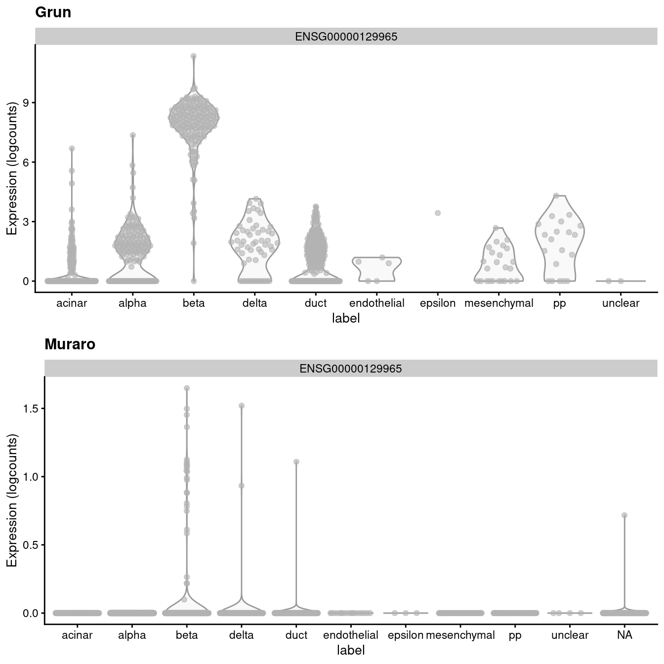
Figure 3.1: Distribution of uncorrected expression values for INS-IGF2 across the cell types in the Grun and Muraro pancreas datasets.
A “perfect” batch correction algorithm must eliminate differences in the expression of this gene between batches. Failing to do so would result in an incomplete merging of cell types - in this case, beta cells - across batches as they would still be separated on the dimension defined by INS-IGF2. Exactly how this is done can vary; Figure 3.2 presents one possible outcome from MNN correction, though another algorithm may choose to align the profiles by setting INS-IGF2 expression to zero for all cells in both batches.
library(batchelor)
set.seed(1011011)
mnn.pancreas <- quickCorrect(grun=sce.grun, muraro=sce.muraro,
    precomputed=list(dec.grun, dec.muraro))

corrected <- mnn.pancreas$corrected
corrected$label <- c(sce.grun$label, sce.muraro$label)
plotExpression(corrected, x="label", features="ENSG00000129965",
exprs_values="reconstructed", other_fields="batch") + facet_wrap(~batch) 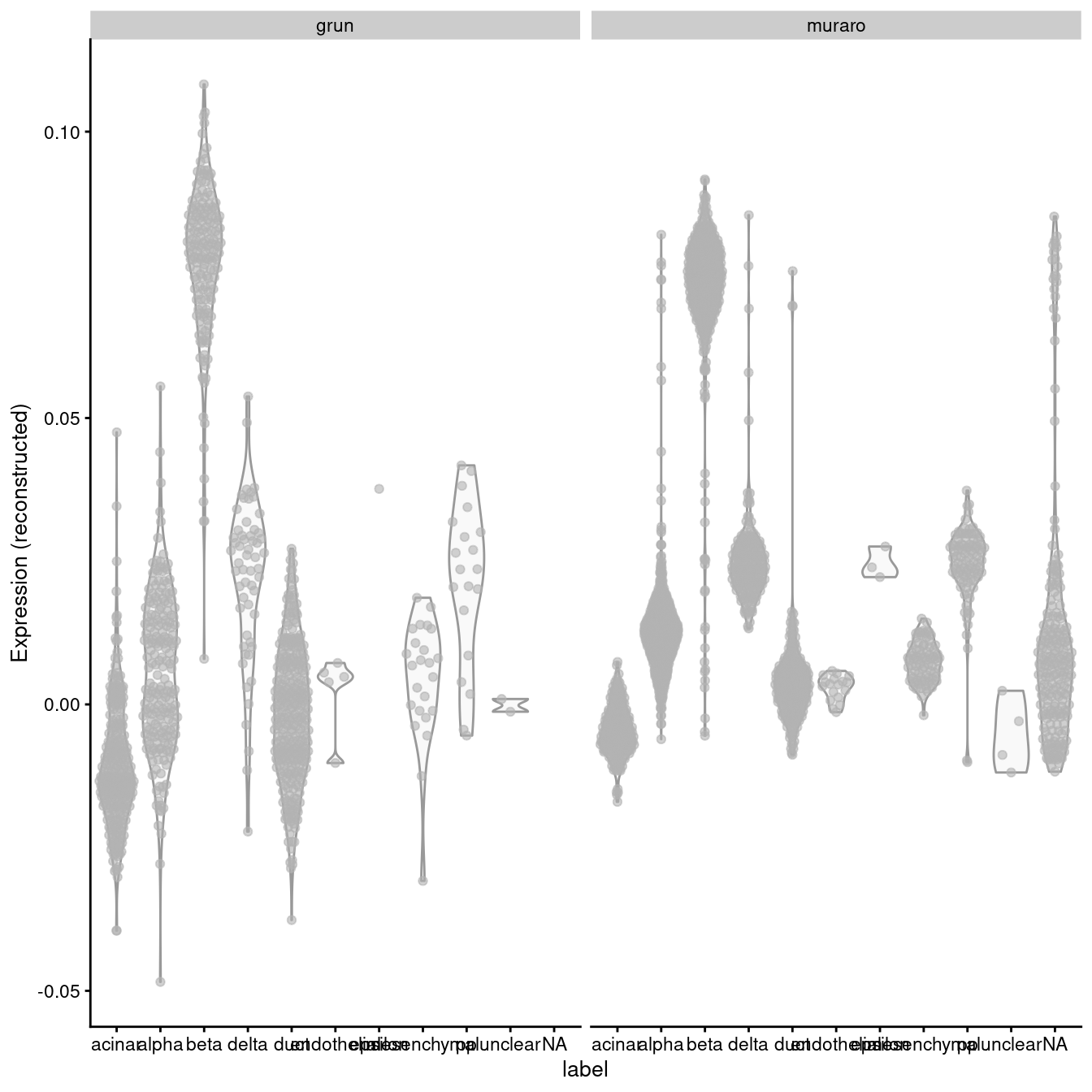
Figure 3.2: Distribution of MNN-corrected expression values for INS-IGF2 across the cell types in the Grun and Muraro pancreas datasets.
In this manner, we have introduced artificial DE between the cell types in the Muraro batch in order to align with the DE present in the Grun dataset. We would be misled into believing that beta cells upregulate INS-IGF2 in both batches when in fact this is only true for the Grun batch. At best, this is only a minor error - after all, we do actually have INS-IGF2-high beta cells, they are just limited to batch 2, which limits the utility of this gene as a general marker. At worst, this can change the conclusions, e.g., if batch 1 was drug-treated and batch 2 was a control, we might mistakenly conclude that our drug has no effect on INS-IGF2 expression in beta cells. (This is discussed further in Section ??.)
3.3 After blocking on the batch
For per-gene analyses that involve comparisons within batches, we prefer to use the uncorrected expression values and blocking on the batch in our statistical model. For marker detection, this is done by performing comparisons within each batch and combining statistics across batches (Basic Section 6.7). This strategy is based on the expectation that any genuine DE between clusters should still be present in a within-batch comparison where batch effects are absent. It penalizes genes that exhibit inconsistent DE across batches, thus protecting against misleading conclusions when a population in one batch is aligned to a similar-but-not-identical population in another batch. We demonstrate this approach below using a blocked \(t\)-test to detect markers in the PBMC dataset, where the presence of the same pattern across clusters within each batch (Figure 3.3) is reassuring.
#--- loading ---#
library(TENxPBMCData)
all.sce <- list(
    pbmc3k=TENxPBMCData('pbmc3k'),
    pbmc4k=TENxPBMCData('pbmc4k'),
    pbmc8k=TENxPBMCData('pbmc8k')
)

#--- quality-control ---#
library(scater)
stats <- high.mito <- list()
for (n in names(all.sce)) {
    current <- all.sce[[n]]
    is.mito <- grep("MT", rowData(current)$Symbol_TENx)
    stats[[n]] <- perCellQCMetrics(current, subsets=list(Mito=is.mito))
    high.mito[[n]] <- isOutlier(stats[[n]]$subsets_Mito_percent, type="higher")
    all.sce[[n]] <- current[,!high.mito[[n]]]
}

#--- normalization ---#
all.sce <- lapply(all.sce, logNormCounts)

#--- variance-modelling ---#
library(scran)
all.dec <- lapply(all.sce, modelGeneVar)
all.hvgs <- lapply(all.dec, getTopHVGs, prop=0.1)

#--- dimensionality-reduction ---#
library(BiocSingular)
set.seed(10000)
all.sce <- mapply(FUN=runPCA, x=all.sce, subset_row=all.hvgs,
    MoreArgs=list(ncomponents=25, BSPARAM=RandomParam()),
    SIMPLIFY=FALSE)

set.seed(100000)
all.sce <- lapply(all.sce, runTSNE, dimred="PCA")

set.seed(1000000)
all.sce <- lapply(all.sce, runUMAP, dimred="PCA")

#--- clustering ---#
for (n in names(all.sce)) {
    g <- buildSNNGraph(all.sce[[n]], k=10, use.dimred='PCA')
    clust <- igraph::cluster_walktrap(g)$membership
    colLabels(all.sce[[n]])  <- factor(clust)
}

#--- data-integration ---#
# Intersecting the common genes.
universe <- Reduce(intersect, lapply(all.sce, rownames))
all.sce2 <- lapply(all.sce, "[", i=universe,)
all.dec2 <- lapply(all.dec, "[", i=universe,)

# Renormalizing to adjust for differences in depth.
library(batchelor)
normed.sce <- do.call(multiBatchNorm, all.sce2)

# Identifying a set of HVGs using stats from all batches.
combined.dec <- do.call(combineVar, all.dec2)
combined.hvg <- getTopHVGs(combined.dec, n=5000)

set.seed(1000101)
merged.pbmc <- do.call(fastMNN, c(normed.sce,
    list(subset.row=combined.hvg, BSPARAM=RandomParam())))

#--- merged-clustering ---#
g <- buildSNNGraph(merged.pbmc, use.dimred="corrected")
colLabels(merged.pbmc) <- factor(igraph::cluster_louvain(g)$membership)
table(colLabels(merged.pbmc), merged.pbmc$batch)
# TODO: make this process a one-liner.
all.sce2 <- lapply(all.sce2, function(x) {
rowData(x) <- rowData(all.sce2[[1]])
x
})
combined <- do.call(cbind, all.sce2)
combined$batch <- rep(c("3k", "4k", "8k"), vapply(all.sce2, ncol, 0L))
clusters.mnn <- colLabels(merged.pbmc)
# Marker detection with block= set to the batch factor.
library(scran)
m.out <- findMarkers(combined, clusters.mnn, block=combined$batch,
direction="up", lfc=1, row.data=rowData(combined)[,3,drop=FALSE])
# Seems like CD8+ T cells:
demo <- m.out[["10"]]
as.data.frame(demo[1:10,c("Symbol", "Top", "p.value", "FDR")]) ## Symbol Top p.value FDR
## ENSG00000172116 CD8B 1 6.165e-101 7.406e-98
## ENSG00000167286 CD3D 1 5.348e-205 1.856e-201
## ENSG00000111716 LDHB 1 4.785e-149 8.790e-146
## ENSG00000213741 RPS29 1 0.000e+00 0.000e+00
## ENSG00000171858 RPS21 1 0.000e+00 0.000e+00
## ENSG00000171223 JUNB 1 1.024e-233 4.569e-230
## ENSG00000177954 RPS27 2 2.482e-294 1.550e-290
## ENSG00000153563 CD8A 2 1.000e+00 1.000e+00
## ENSG00000124614 RPS10 2 0.000e+00 0.000e+00
## ENSG00000198851 CD3E 2 1.518e-173 3.161e-170plotExpression(combined, x=I(factor(clusters.mnn)), swap_rownames="Symbol",
features=c("CD3D", "CD8B"), colour_by="batch") + facet_wrap(Feature~colour_by)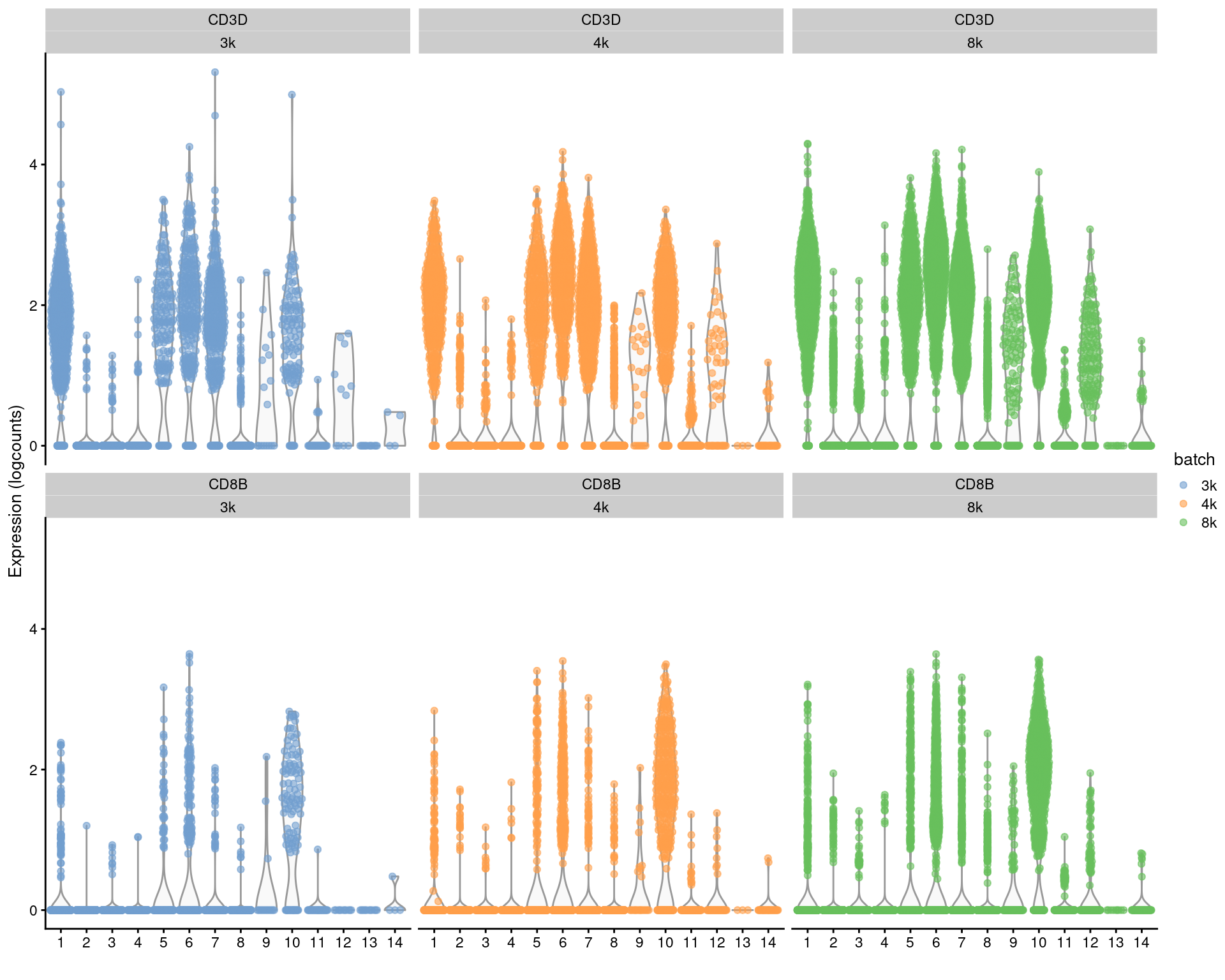
Figure 3.3: Distributions of uncorrected log-expression values for CD8B and CD3D within each cluster in each batch of the merged PBMC dataset.
In contrast, we suggest limiting the use of per-gene corrected values to visualization, e.g., when coloring points on a \(t\)-SNE plot by per-cell expression. This can be more aesthetically pleasing than uncorrected expression values that may contain large shifts on the colour scale between cells in different batches. Use of the corrected values in any quantitative procedure should be treated with caution, and should be backed up by similar results from an analysis on the uncorrected values.
3.4 For between-batch comparisons
Here, the main problem is that correction will inevitably introduce artificial agreement across batches. Removal of biological differences between batches in the corrected data is unavoidable if we want to mix cells from different batches. To illustrate, we shall consider the pancreas dataset from Segerstolpe et al. (2016), involving both healthy and diabetic donors. Each donor has been treated as a separate batch for the purpose of removing donor effects.
#--- loading ---#
library(scRNAseq)
sce.seger <- SegerstolpePancreasData()

#--- gene-annotation ---#
library(AnnotationHub)
edb <- AnnotationHub()[["AH73881"]]
symbols <- rowData(sce.seger)$symbol
ens.id <- mapIds(edb, keys=symbols, keytype="SYMBOL", column="GENEID")
ens.id <- ifelse(is.na(ens.id), symbols, ens.id)

# Removing duplicated rows.
keep <- !duplicated(ens.id)
sce.seger <- sce.seger[keep,]
rownames(sce.seger) <- ens.id[keep]

#--- sample-annotation ---#
emtab.meta <- colData(sce.seger)[,c("cell type", "disease",
    "individual", "single cell well quality")]
colnames(emtab.meta) <- c("CellType", "Disease", "Donor", "Quality")
colData(sce.seger) <- emtab.meta

sce.seger$CellType <- gsub(" cell", "", sce.seger$CellType)
sce.seger$CellType <- paste0(
    toupper(substr(sce.seger$CellType, 1, 1)),
    substring(sce.seger$CellType, 2))

#--- quality-control ---#
low.qual <- sce.seger$Quality == "low quality cell"

library(scater)
stats <- perCellQCMetrics(sce.seger)
qc <- quickPerCellQC(stats, percent_subsets="altexps_ERCC_percent",
    batch=sce.seger$Donor,
    subset=!sce.seger$Donor %in% c("HP1504901", "HP1509101"))

sce.seger <- sce.seger[,!(qc$discard | low.qual)]

#--- normalization ---#
library(scran)
clusters <- quickCluster(sce.seger)
sce.seger <- computeSumFactors(sce.seger, clusters=clusters)
sce.seger <- logNormCounts(sce.seger)

#--- variance-modelling ---#
for.hvg <- sce.seger[,librarySizeFactors(altExp(sce.seger)) > 0 & sce.seger$Donor!="AZ"]
dec.seger <- modelGeneVarWithSpikes(for.hvg, "ERCC", block=for.hvg$Donor)
chosen.hvgs <- getTopHVGs(dec.seger, n=2000)

#--- dimensionality-reduction ---#
library(BiocSingular)
set.seed(101011001)
sce.seger <- runPCA(sce.seger, subset_row=chosen.hvgs, ncomponents=25)
sce.seger <- runTSNE(sce.seger, dimred="PCA")

#--- clustering ---#
library(bluster)
clust.out <- clusterRows(reducedDim(sce.seger, "PCA"), NNGraphParam(), full=TRUE)
snn.gr <- clust.out$objects$graph
colLabels(sce.seger) <- clust.out$clusters

#--- data-integration ---#
library(batchelor)

set.seed(10001010)
corrected <- fastMNN(sce.seger, batch=sce.seger$Donor, subset.row=chosen.hvgs)

set.seed(10000001)
corrected <- runTSNE(corrected, dimred="corrected")

colLabels(corrected) <- clusterRows(reducedDim(corrected, "corrected"), NNGraphParam())

tab <- table(Cluster=colLabels(corrected), Donor=corrected$batch)
tab## class: SingleCellExperiment
## dim: 25454 2090
## metadata(0):
## assays(2): counts logcounts
## rownames(25454): ENSG00000118473 ENSG00000142920 ... ENSG00000278306
## eGFP
## rowData names(2): symbol refseq
## colnames(2090): HP1502401_H13 HP1502401_J14 ... HP1526901T2D_N8
## HP1526901T2D_A8
## colData names(6): CellType Disease ... sizeFactor label
## reducedDimNames(2): PCA TSNE
## mainExpName: endogenous
## altExpNames(1): ERCCWe examine the expression of INS in beta cells across donors (Figure 3.4). We observe some variation across donors with a modest downregulation in the set of diabetic patients.
library(scater)
sce.beta <- sce.seger[,sce.seger$CellType=="Beta"]
by.cell <- plotExpression(sce.beta, features="INS", swap_rownames="symbol", colour_by="Disease",
    # Arrange donors by disease status, for a prettier plot.
    x=I(reorder(sce.beta$Donor, sce.beta$Disease, FUN=unique)))

ave.beta <- aggregateAcrossCells(sce.beta, statistics="mean",
    use.assay.type="logcounts", ids=sce.beta$Donor, use.altexps=FALSE)
by.sample <- plotExpression(ave.beta, features="INS", swap_rownames="symbol",
    x="Disease", colour_by="Disease")

gridExtra::grid.arrange(by.cell, by.sample, ncol=2)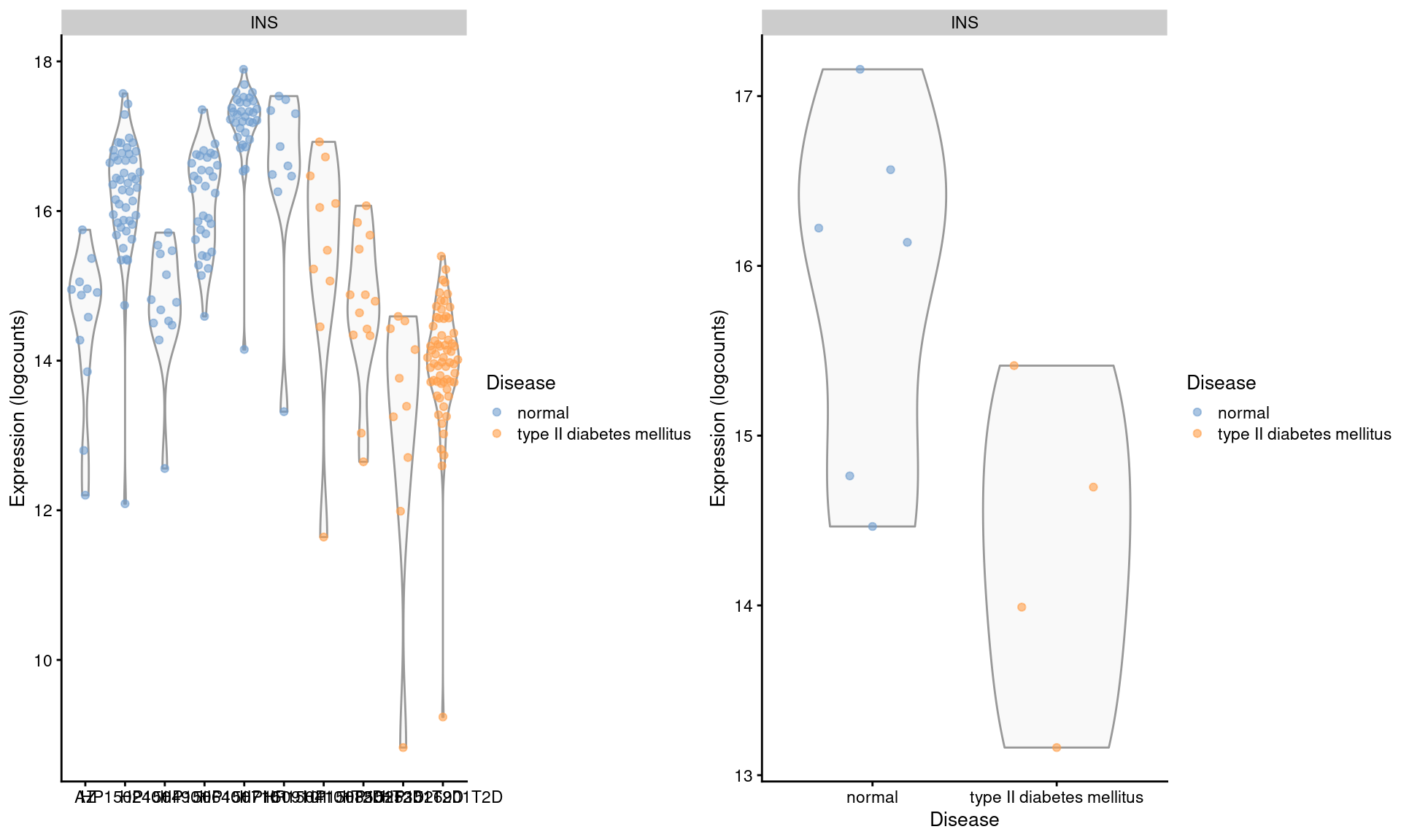
Figure 3.4: Distribution of log-expression values for INS in beta cells across donors in the Segerstolpe pancreas dataset. Each point represents a cell in each donor (left) or the average of all cells in each donor (right), and is colored according to disease status of the donor.
We repeat this examination on the MNN-corrected values, where the relative differences are largely eliminated (Figure 3.5). Note that the change in the y-axis scale can largely be ignored as the corrected values are on a different scale after cosine normalization.
corr.beta <- corrected[,sce.seger$CellType=="Beta"]
corr.beta$Donor <- sce.beta$Donor
corr.beta$Disease <- sce.beta$Disease
by.cell <- plotExpression(corr.beta, features="ENSG00000254647",
    x=I(reorder(sce.beta$Donor, sce.beta$Disease, FUN=unique)),
    exprs_values="reconstructed", colour_by="Disease")

ave.beta <- aggregateAcrossCells(corr.beta, statistics="mean",
    use.assay.type="reconstructed", ids=sce.beta$Donor)
by.sample <- plotExpression(ave.beta, features="ENSG00000254647",
    exprs_values="reconstructed", x="Disease", colour_by="Disease")

gridExtra::grid.arrange(by.cell, by.sample, ncol=2)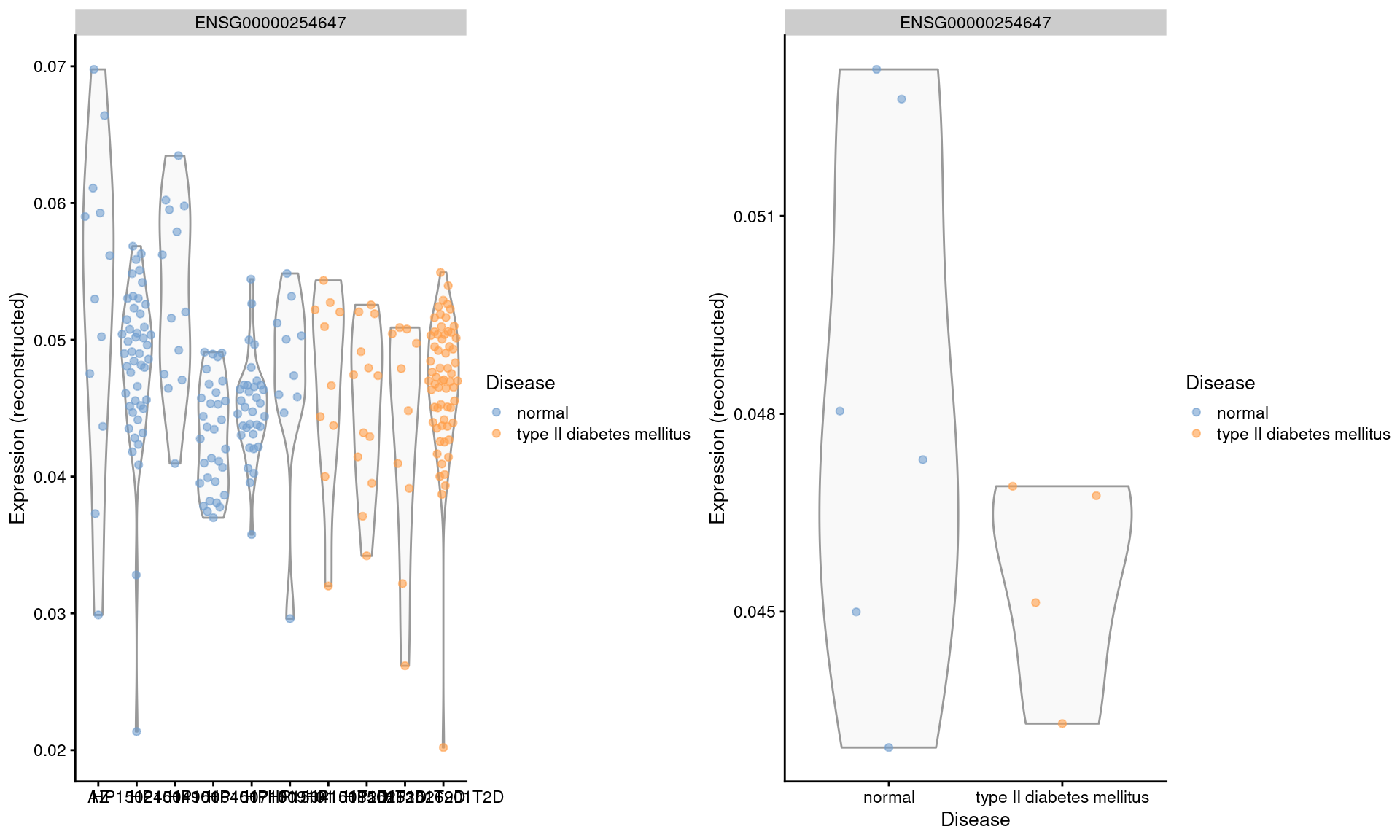
Figure 3.5: Distribution of MNN-corrected log-expression values for INS in beta cells across donors in the Segerstolpe pancreas dataset. Each point represents a cell in each donor (left) or the average of all cells in each donor (right), and is colored according to disease status of the donor.
We will not attempt to determine whether the INS downregulation represents genuine biology or a batch effect (see Workflow Section 8.9 for a formal analysis). The real issue is that the analyst never has a chance to consider this question when the corrected values are used. Moreover, the variation in expression across donors is understated, which is problematic if we want to make conclusions about population variability.
We suggest performing cross-batch comparisons on the original expression values wherever possible (Chapter 4). Rather than performing correction, we rely on the statistical model to account for batch-to-batch variation when making inferences. This preserves any differences between conditions and does not distort the variance structure. Some further consequences of correction in the context of multi-condition comparisons are discussed in Section 6.4.2.
Session Info
R version 4.2.0 (2022-04-22)
Platform: x86_64-pc-linux-gnu (64-bit)
Running under: Ubuntu 20.04.4 LTS

Matrix products: default
BLAS:   /home/biocbuild/bbs-3.15-bioc/R/lib/libRblas.so
LAPACK: /home/biocbuild/bbs-3.15-bioc/R/lib/libRlapack.so

locale:
 [1] LC_CTYPE=en_US.UTF-8       LC_NUMERIC=C
 [3] LC_TIME=en_GB              LC_COLLATE=C
 [5] LC_MONETARY=en_US.UTF-8    LC_MESSAGES=en_US.UTF-8
 [7] LC_PAPER=en_US.UTF-8       LC_NAME=C
 [9] LC_ADDRESS=C               LC_TELEPHONE=C
[11] LC_MEASUREMENT=en_US.UTF-8 LC_IDENTIFICATION=C

attached base packages:
[1] stats4    stats     graphics  grDevices utils     datasets  methods
[8] base

other attached packages:
 [1] scran_1.24.0                HDF5Array_1.24.0
 [3] rhdf5_2.40.0                DelayedArray_0.22.0
 [5] Matrix_1.4-1                batchelor_1.12.0
 [7] scater_1.24.0               ggplot2_3.3.6
 [9] scuttle_1.6.2               SingleCellExperiment_1.18.0
[11] SingleR_1.10.0              SummarizedExperiment_1.26.1
[13] Biobase_2.56.0              GenomicRanges_1.48.0
[15] GenomeInfoDb_1.32.2         IRanges_2.30.0
[17] S4Vectors_0.34.0            BiocGenerics_0.42.0
[19] MatrixGenerics_1.8.0        matrixStats_0.62.0
[21] BiocStyle_2.24.0            rebook_1.6.0

loaded via a namespace (and not attached):
 [1] ggbeeswarm_0.6.0          colorspace_2.0-3
 [3] ellipsis_0.3.2            bluster_1.6.0
 [5] XVector_0.36.0            BiocNeighbors_1.14.0
 [7] farver_2.1.0              ggrepel_0.9.1
 [9] fansi_1.0.3               codetools_0.2-18
[11] sparseMatrixStats_1.8.0   knitr_1.39
[13] jsonlite_1.8.0            ResidualMatrix_1.6.0
[15] cluster_2.1.3             graph_1.74.0
[17] BiocManager_1.30.18       compiler_4.2.0
[19] dqrng_0.3.0               assertthat_0.2.1
[21] fastmap_1.1.0             limma_3.52.1
[23] cli_3.3.0                 BiocSingular_1.12.0
[25] htmltools_0.5.2           tools_4.2.0
[27] rsvd_1.0.5                igraph_1.3.1
[29] gtable_0.3.0              glue_1.6.2
[31] GenomeInfoDbData_1.2.8    dplyr_1.0.9
[33] rappdirs_0.3.3            Rcpp_1.0.8.3
[35] jquerylib_0.1.4           vctrs_0.4.1
[37] rhdf5filters_1.8.0        DelayedMatrixStats_1.18.0
[39] xfun_0.31                 stringr_1.4.0
[41] beachmat_2.12.0           lifecycle_1.0.1
[43] irlba_2.3.5               statmod_1.4.36
[45] XML_3.99-0.9              edgeR_3.38.1
[47] zlibbioc_1.42.0           scales_1.2.0
[49] parallel_4.2.0            yaml_2.3.5
[51] gridExtra_2.3             sass_0.4.1
[53] stringi_1.7.6             highr_0.9
[55] ScaledMatrix_1.4.0        filelock_1.0.2
[57] BiocParallel_1.30.2       rlang_1.0.2
[59] pkgconfig_2.0.3           bitops_1.0-7
[61] evaluate_0.15             lattice_0.20-45
[63] purrr_0.3.4               Rhdf5lib_1.18.2
[65] CodeDepends_0.6.5         labeling_0.4.2
[67] cowplot_1.1.1             tidyselect_1.1.2
[69] magrittr_2.0.3            bookdown_0.26
[71] R6_2.5.1                  generics_0.1.2
[73] metapod_1.4.0             DBI_1.1.2
[75] pillar_1.7.0              withr_2.5.0
[77] RCurl_1.98-1.6            tibble_3.1.7
[79] dir.expiry_1.4.0          crayon_1.5.1
[81] utf8_1.2.2                rmarkdown_2.14
[83] viridis_0.6.2             locfit_1.5-9.5
[85] grid_4.2.0                digest_0.6.29
[87] munsell_0.5.0             beeswarm_0.4.0
[89] viridisLite_0.4.0         vipor_0.4.5
[91] bslib_0.3.1
References
Grun, D., M. J. Muraro, J. C. Boisset, K. Wiebrands, A. Lyubimova, G. Dharmadhikari, M. van den Born, et al. 2016. “De Novo Prediction of Stem Cell Identity using Single-Cell Transcriptome Data.” Cell Stem Cell 19 (2): 266–77.
Muraro, M. J., G. Dharmadhikari, D. Grun, N. Groen, T. Dielen, E. Jansen, L. van Gurp, et al. 2016. “A Single-Cell Transcriptome Atlas of the Human Pancreas.” Cell Syst 3 (4): 385–94.
Segerstolpe, A., A. Palasantza, P. Eliasson, E. M. Andersson, A. C. Andreasson, X. Sun, S. Picelli, et al. 2016. “Single-Cell Transcriptome Profiling of Human Pancreatic Islets in Health and Type 2 Diabetes.” Cell Metab. 24 (4): 593–607.