Chapter 5 Normalizing for technical biases
5.1 Overview
The complexity of the ChIP-seq technique gives rise to a number of different biases in the data. For a DB analysis, library-specific biases are of particular interest as they can introduce spurious differences between conditions. This includes composition biases, efficiency biases and trended biases. Thus, normalization between libraries is required to remove these biases prior to any statistical analysis.
Several normalization strategies are presented here, though users should only pick one to use for any given analysis. Advice on choosing the most appropriate method is scattered throughout the chapter.
5.2 Eliminating composition biases
5.2.1 Using the TMM method on binned counts
As the name suggests, composition biases are formed when there are differences in the composition of sequences across libraries. Highly enriched regions consume more sequencing resources and thereby suppress the representation of other regions. Differences in the magnitude of suppression between libraries can lead to spurious DB calls. Scaling by library size fails to correct for this as composition biases can still occur in libraries of the same size.
To remove composition biases in csaw, reads are counted into large bins and the counts are used for normalization with the normFactors() wrapper function.
This uses the trimmed mean of M-values (TMM) method (Robinson and Oshlack 2010) to correct for any systematic fold change in the coverage of the bins.
The assumption here is that most bins represent non-DB background regions, so any consistent difference across bins must be technical bias.
#--- loading-files ---#
library(chipseqDBData)
tf.data <- NFYAData()
tf.data
bam.files <- head(tf.data$Path, -1) # skip the input.
bam.files

#--- counting-windows ---#
library(csaw)
frag.len <- 110
win.width <- 10
param <- readParam(minq=20)
data <- windowCounts(bam.files, ext=frag.len, width=win.width, param=param)

#--- filtering ---#
binned <- windowCounts(bam.files, bin=10000, param=param)
fstats <- filterWindowsGlobal(data, binned)
filtered.data <- data[fstats$filter > log2(5),]library(csaw)
binned <- windowCounts(bam.files, bin=TRUE, width=10000, param=param)
filtered.data <- normFactors(binned, se.out=filtered.data)
filtered.data$norm.factors## [1] 1.0084 0.9751 1.0136 1.0033The TMM method trims away putative DB bins (i.e., those with extreme M-values) and computes normalization factors from the remainder to use in edgeR. The size of each library is scaled by the corresponding factor to obtain an effective library size for modelling. A larger normalization factor results in a larger effective library size and is conceptually equivalent to scaling each individual count downwards, given that the ratio of that count to the (effective) library size will be smaller. Check out the edgeR user’s guide for more information.
To elaborate on the above code: the normFactors() call computes normalization factors from the bin-level counts in binned (see Section 5.2.2).
The se.out argument directs the function to return a modified version of filtered.data, where the normalization factors are stored alongside the window-level counts for further analysis.
Composition biases affect both bin- and window-level counts, so computing normalization factors from the former and applying them to the latter is valid -
provided that the library sizes are the same between the two sets of counts, as the factors are interpreted with respect to the library sizes.
(In csaw, separate calls to windowCounts() with the same readParam object will always yield the same library sizes in totals.)
Note that normFactors() skips the precision weighting step in the TMM method.
Weighting aims to increase the contribution of bins with high counts, as these yield more precise M-values.
However, high-abundance bins are more likely to contain binding sites and thus are more likely to be DB compared to background regions.
If any DB regions should survive trimming, upweighting them would be counterproductive.
5.2.2 Motivating the use of large bins
By definition, read coverage is low for background regions of the genome. This can result in a large number of zero counts and undefined M-values when reads are counted into small windows. Adding a prior count is only a superficial solution as the chosen prior will have undue influence on the estimate of the normalization factor when many counts are low. The variance of the fold change distribution is also higher for low counts, which reduces the effectiveness of the trimming procedure. These problems can be overcome by using large bins to increase the size of the counts, thus improving the precision of TMM normalization. The normalization factors computed from the bin-level counts are then applied to the window-level counts of interest.
Of course, this strategy requires the user to supply a bin size. If the bins are too large, background and enriched regions will be included in the same bin. This makes it difficult to trim away bins corresponding to enriched regions. On the other hand, the counts will be too low if the bins are too small. Testing multiple bin sizes is recommended to ensure that the estimates are robust to any changes. A value of 10 kbp is usually suitable for most datasets.
demo <- windowCounts(bam.files, bin=TRUE, width=5000, param=param)
normFactors(demo, se.out=FALSE) # se.out=FALSE to report factors directly.
## [1] 1.0083 0.9779 1.0109 1.0032## [1] 1.0085 0.9723 1.0160 1.0037Here, the factors are consistently close to unity, which suggests that composition bias is negligble in this dataset. See Section~ for some examples with greater bias.
5.2.3 Visualizing normalization with MA plots
The effectiveness of normalization can be examined using a MA plot (Figure 5.1). A single main cloud of points should be present, consisting primarily of background regions. Separation into multiple discrete points indicates that the counts are too low and that larger bin sizes should be used. Composition biases manifest as a vertical shift in the position of this cloud. Ideally, the log-ratios of the corresponding normalization factors should pass through the centre of the cloud. This indicates that undersampling has been identified and corrected.
library(edgeR)
adj.counts <- cpm(asDGEList(binned), log=TRUE)
normfacs <- filtered.data$norm.factors

par(mfrow=c(1, 3), mar=c(5, 4, 2, 1.5))
for (i in seq_len(length(bam.files)-1)) {
    cur.x <- adj.counts[,1]
    cur.y <- adj.counts[,1+i]
    smoothScatter(x=(cur.x+cur.y)/2+6*log2(10), y=cur.x-cur.y,
        xlab="A", ylab="M", main=paste("1 vs", i+1))
    all.dist <- diff(log2(normfacs[c(i+1, 1)]))
    abline(h=all.dist, col="red")
}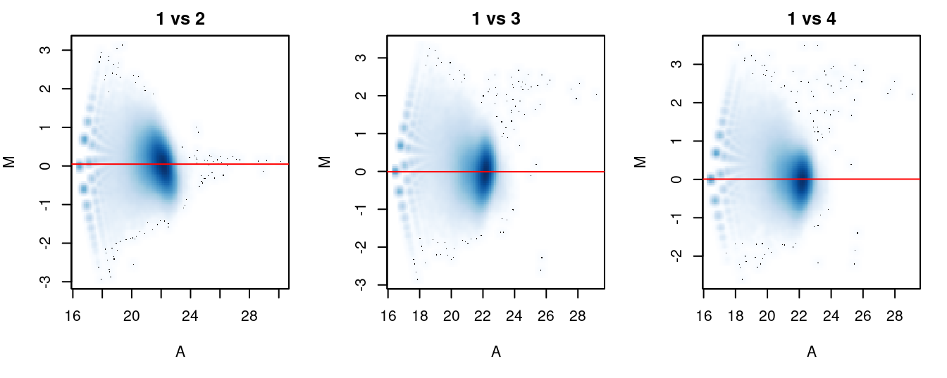
Figure 5.1: MA plots for each sample compared to the first in the NF-YA dataset. Each point represents a 10 kbp bin and the red line denotes the scaled normalization factor for each sample.
5.3 Eliminating efficiency biases
5.3.0.1 Using TMM on high-abundance regions
Efficiency biases in ChIP-seq data refer to fold changes in enrichment that are introduced by variability in IP efficiencies between libraries. These technical differences are not biologically interesting and must be removed. This can be achieved by assuming that high-abundance windows contain binding sites. Consider the following H3K4me3 data set, where reads are counted into 150 bp windows.
## DataFrame with 4 rows and 3 columns
##                   Name            Description      Path
##            <character>            <character>    <List>
## 1    h3k4me3-proB-8110   pro-B H3K4me3 (8110) <BamFile>
## 2    h3k4me3-proB-8115   pro-B H3K4me3 (8115) <BamFile>
## 3 h3k4me3-matureB-8070 mature B H3K4me3 (80.. <BamFile>
## 4 h3k4me3-matureB-8088 mature B H3K4me3 (80.. <BamFile>
me.files <- k4data$Path[c(1,3)] # just one sample from each condition, for brevity.
me.demo <- windowCounts(me.files, width=150, param=param)High-abundance windows are chosen using a global filtering approach described in Section @ref{sec:global-filter}.
Here, the binned counts in me.bin are only used for defining the background abundance, not for computing normalization factors.
me.bin <- windowCounts(me.files, bin=TRUE, width=10000, param=param)
keep <- filterWindowsGlobal(me.demo, me.bin)$filter > log2(3)
filtered.me <- me.demo[keep,]
The TMM method is then applied to eliminate systematic differences across those windows. This assumes that most binding sites in the genome are not DB - thus, any systematic differences in coverage among the high-abundance windows must be caused by differences in IP efficiency between libraries or some other technical issue. Scaling by the normalization factors will subseqeuently remove these biases prior to further analyses.
## [1] 1.2655 0.7902The downside of this approach is that genuine biological differences may be removed when the assumption of a non-DB majority does not hold, e.g., overall binding is truly lower in one condition. In such cases, it is safer to normalize for composition biases - see Section 5.4 for a discussion of the choice between normalization methods.
While the above process seems rather involved, this is only because we need to work our way through counting and filtering for a new data set.
Only normFactors() is actually needed for the normalization step.
As a demonstration, we repeat this procedure on another data set involving H3 acetylation.
acdata <- H3K9acData()
ac.files <- acdata$Path[c(1,2)] # subsetting again for brevity.

# Counting:
ac.demo <- windowCounts(ac.files, width=150, param=param)

# Filtering:
ac.bin <- windowCounts(ac.files, bin=TRUE, width=10000, param=param)
keep <- filterWindowsGlobal(ac.demo, ac.bin)$filter > log2(5)
filtered.ac <- ac.demo[keep,]

# Normalization:
filtered.ac <- normFactors(filtered.ac, se.out=TRUE)
ac.eff <- filtered.ac$norm.factors
ac.eff
## [1] 1.0746 0.93065.3.1 Filtering windows prior to normalization
Normalization for efficiency biases is performed on window-level counts instead of bin counts. This is possible as filtering ensures that we only retain the high-abundance windows, i.e., those with counts that are large enough for stable calculation of normalization factors. It is not necessary to use larger windows or bins, and indeed, direct use of the windows of interest ensures removal of systematic differences in those windows prior to downstream analyses.
The filtering procedure needs to be stringent enough to avoid retaining windows from background regions. These will interfere with calculation of normalization factors from binding sites. This is due to the lower coverage for background regions, as well as the fact that they are not affected by efficiency bias (and cannot contribute to its estimation). Conversely, attempting to use the factors computed from high-abundance windows on windows from background regions will result in incorrect normalization of the latter. Thus, it is usually better to err on the side of caution and filter aggressively to ensure that background regions are not retained in downstream analyses. Obviously, though, retaining too few windows will result in unstable estimates of the normalization factors.
5.3.2 Visualizing normalization with MA plots
We again visualize the effect of normalization with MA plots. We continue to use the counts for 10 kbp bins to construct the plots, rather than with those from the windows. This is useful as the behavior of the entire genome can be examined, rather than just that of the high-abundance windows. It also allows calculation of and comparison to the factors for composition bias.
# Again, just setting se.out=FALSE to report factors directly.
me.comp <- normFactors(me.bin, se.out=FALSE)
me.comp
## [1] 0.7751 1.2902## [1] 0.9474 1.0556In Figure 5.2, the clouds at low and high A-values represent the background and bound regions, respectively. The normalization factors from removal of composition bias (dashed) pass through the former, whereas the factors to remove efficiency bias (full) pass through the latter. A non-zero M-value location for the high A-value cloud represents a systematic difference between libraries for the bound regions, either due to genuine DB or variable IP efficiency. This also induces composition bias, leading to a non-zero M-value for the background cloud.
par(mfrow=c(1,2))
for (main in c("H3K4me3", "H3ac")) {
    if (main=="H3K4me3") {
        bins <- me.bin
        comp <- me.comp
        eff <- me.eff
    } else {
        bins <- ac.bin
        comp <- ac.comp
        eff <- ac.eff
    }
    adjc <- cpm(asDGEList(bins), log=TRUE)
    smoothScatter(x=rowMeans(adjc), y=adjc[,1]-adjc[,2],
                  xlab="A", ylab="M", main=main)
    abline(h=log2(eff[1]/eff[2]), col="red")
    abline(h=log2(comp[1]/comp[2]), col="red", lty=2)
}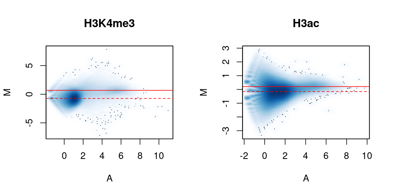
Figure 5.2: MA plots between individual samples in the H3K4me3 and H3ac datasets. Each point represents a 10 kbp bin and the red lines denotes the ratio of normalization factors computed from bins (dashed) or high-abundance windows (full).
5.4 Choosing between normalization strategies
The normalization strategies for composition and efficiency biases are mutually exclusive, as only one set of normalization factors will ultimately be used in edgeR. The choice between the two methods depends on whether one assumes that the systematic differences at high abundances represent genuine DB events. If so, the binned TMM method from Section 5.2 should be used to remove composition bias. This will preserve the assumed DB, at the cost of ignoring any efficiency biases that might be present. Otherwise, if the systematic differences are not genuine DB, they must represent efficiency bias and should be removed by applying the TMM method on high-abundance windows (Section 5.3). Some understanding of the biological context is useful in making this decision, e.g., comparing a wild-type against a knock-out for the target protein should result in systematic DB, while overall levels of histone marking are expected to be consistent in most conditions.
For the main NF-YA example, there is no expectation of constant binding between cell types. Thus, normalization factors will be computed to remove composition biases. This ensures that any genuine systematic changes in binding will still be picked up. In general, normalization for composition bias is a good starting point for any analysis. This can be considered as the “default” strategy unless there is evidence for a confounding efficiency bias.
5.5 With spike-in chromatin
Some studies use spike-in chromatin for scaling normalization of ChIP-seq data (Bonhoure et al. 2014; Orlando et al. 2014). Briefly, a constant amount of chromatin from a different species is added to each sample at the start of the ChIP-seq protocol. The mixture is processed and sequenced in the usual manner, using antibodies that can bind epitopes of interest from both species. The coverage of the spiked-in foreign chromatin is then quantified in each library. As the quantity of foreign chromatin should be constant in each sample, the coverage of binding sites on the foreign genome should also be the same between libraries. Any difference in coverage between libraries represents some technical bias that should be removed by scaling.
This normalization strategy can be implemented in csaw with some work.
Assuming that the reference genome includes appropriate sequences from the foreign genome, coverage is quantified across genomic windows with windowCounts().
Filtering is performed to select for high-abundance windows in the foreign genome, yielding counts for all enriched spike-in regions.
(The filtered object is named spike.data in the code below.)
Normalization factors are computed by applying the TMM method on these counts via normFactors().
This aims to identify the fold-change in coverage between samples that is attributable to technical effects.
# Pretend chr1 is a spike-in, for demonstration purposes only!
# TODO: find an actual spike-in dataset and get it into chipseqDBData.
is.1 <- seqnames(rowRanges(filtered.data))=="chr1"
spike.data <- filtered.data[is.1,]
endog.data <- filtered.data[!is.1,]

endog.data <- normFactors(spike.data, se.out=endog.data)
In the code above, the spike-in normalization factors are returned in a modified copy of endog.data for further analysis of the endogenous windows.
We assume that the library sizes in totals are the same between spike.data and endog.data,
which should be the case if they were formed by subsetting the output of a single windowCounts() call.
This ensures that the normalization factors computed from the spike-in windows are applicable to the endogenous windows.
Compared to the previous normalization methods, the spike-in approach does not distinguish between composition and efficiency biases. Instead, it uses the fold-differences in the coverage of spiked-in binding sites to empirically measure and remove the net bias between libraries. This avoids the need for assumptions regarding the origin of any systematic differences between libraries. That said, spike-in normalization involves some strong assumptions of its own. In particular, the ratio of spike-in chromatin to endogenous chromatin is assumed to be the same in each sample. This requires accurate quantitation of the chromatin in each sample, followed by precise addition of small spike-in quantities. Furthermore, the spike-in chromatin, its protein target and the corresponding antibody are assumed to behave in the same manner as their endogenous counterparts throughout the ChIP-seq protocol. Whether these assumptions are reasonable will depend on the experimenter and the nature of the spike-in chromatin.
5.6 Dealing with trended biases
In more extreme cases, the bias may vary with the average abundance to form a trend. One possible explanation is that changes in IP efficiency will have little effect at low-abundance background regions and more effect at high-abundance binding sites. Thus, the magnitude of the bias between libraries will change with abundance. The trend cannot be corrected with scaling methods as no single scaling factor will remove differences at all abundances. Rather, non-linear methods are required, such as cyclic loess or quantile normalization.
One such implementation of a non-linear normalization method is provided in normOffsets().
This is based on the fast loess algorithm (Ballman et al. 2004) with minor adaptations to handle low counts.
A matrix is produced that contains an offset term for each bin/window in each library.
This offset matrix can then be directly used in edgeR, assuming that the bins or windows used in normalization are also the ones to be tested for DB.
We demonstrate this procedure below, using filtered counts for 2 kbp windows in the H3 acetylation data set.
(This window size is chosen purely for aesthetics in this demonstration, as the trend is less obvious at smaller widths.
Obviously, users should pick a more appropriate value for their analysis.)
ac.demo2 <- windowCounts(ac.files, width=2000L, param=param)

# Filtering for high-abundance intervals.
filtered <- filterWindowsGlobal(ac.demo2, ac.bin)
keep <- filtered$filter > log2(4)
ac.demo2 <- ac.demo2[keep,]

# Actually applying the normalization.
ac.demo2 <- normOffsets(ac.demo2)
ac.off <- assay(ac.demo2, "offset")
head(ac.off)
## [,1] [,2]
## [1,] 15.95 15.8
## [2,] 15.95 15.8
## [3,] 15.95 15.8
## [4,] 15.95 15.8
## [5,] 15.95 15.8
## [6,] 15.95 15.8By default, the offsets are stored in the RangedSummarizedExperiment object as an "offset" entry in the assays slot.
Each offset represents the log-transformed scaling factor that needs to be applied to the corresponding entry of the count matrix for its normalization.
Any operations like subsetting that are applied to modify the object will also be applied to the offsets, allowing for synchronised processing.
Functions from packages like edgeR will also respect the offsets during model fitting.
We again examine the MA plots in Figure 5.3 to determine whether normalization was successful. Any abundance-dependent trend in the M-values should be eliminated after applying the offsets to the log-counts. This is done by subtraction, though note that the offsets are base \(e\) while most log-values in edgeR are reported as base 2.
par(mfrow=c(1,2))

# MA plot without normalization.
ac.y <- asDGEList(ac.demo2)
lib.size <- ac.y$samples$lib.size
adjc <- cpm(ac.y, log=TRUE)
abval <- aveLogCPM(ac.y)
mval <- adjc[,1]-adjc[,2]

fit <- loessFit(x=abval, y=mval)
smoothScatter(abval, mval, ylab="M", xlab="Average logCPM",
    main="Raw", ylim=c(-2,2), xlim=c(0, 7))
o <- order(abval)
lines(abval[o], fit$fitted[o], col="red")

# Repeating after normalization.
re.adjc <- log2(assay(ac.demo2)+0.5) - ac.off/log(2)
mval <- re.adjc[,1]-re.adjc[,2]

fit <- loessFit(x=abval, y=mval)
smoothScatter(abval, re.adjc[,1]-re.adjc[,2], ylab="M", xlab="Average logCPM",
    main="Normalized", ylim=c(-2,2), xlim=c(0, 7))
lines(abval[o], fit$fitted[o], col="red")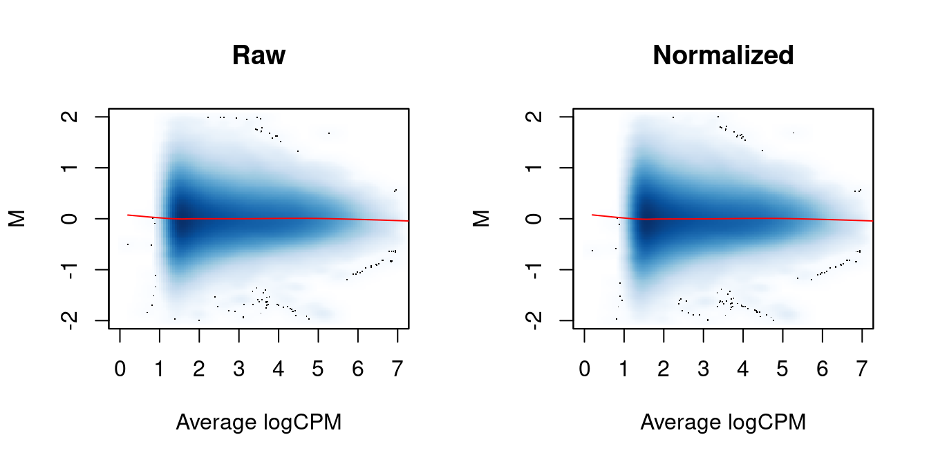
Figure 5.3: MA plots between individual samples in the H3ac dataset before and after trended normalization. Each point represents a 2 kbp bin, and the trend represents a fitted loess curve.
Loess normalization of trended biases is quite similar to TMM normalization for efficiency biases described in Section 5.3. Both methods assume a non-DB majority across features, and will not be appropriate if there is a change in overall binding. Loess normalization involves a slightly stronger assumption of a non-DB majority at every abundance, not just across all bound regions. This is necessary to remove trended biases but may also discard genuine changes, such as a subset of DB sites at very high abundances.
Compared to TMM normalization, the accuracy of loess normalization is less dependent on stringent filtering.
This is because the use of a trend accommodates changes in the bias between high-abundance binding sites and low-abundance background regions.
Nonetheless, some filtering is still necessary to avoid inaccuracies in loess fitting at low abundances.
Any filter statistic for the windows should be based on the average abundance from aveLogCPM(), such as those calculated using filterWindowsGlobal() or equivalents.
An average abundance threshold will act as a clean vertical cutoff in the MA plots above.
This avoids introducing spurious trends at the filter boundary that might affect normalization.
5.7 A word on other biases
No normalization is performed to adjust for differences in mappability or sequencability between different regions of the genome. Region-specific biases are assumed to be constant between libraries. This is generally reasonable as the biases depend on fixed properties of the genome sequence such as GC content. Thus, biases should cancel out during DB comparisons. Any variability between samples will just be absorbed into the dispersion estimate.
That said, explicit normalization to correct these biases can improve results for some datasets. Procedures like GC correction could decrease the observed variability by removing systematic differences between replicates. Of course, this also assumes that the targeted differences have no biological relevance. Detection power may be lost if this is not true. For example, differences in the GC content distribution can be driven by technical bias as well as biology, e.g., when protein binding is associated with a specific GC composition.
Session information
R version 4.1.0 (2021-05-18)
Platform: x86_64-pc-linux-gnu (64-bit)
Running under: Ubuntu 20.04.2 LTS

Matrix products: default
BLAS:   /home/biocbuild/bbs-3.13-bioc/R/lib/libRblas.so
LAPACK: /home/biocbuild/bbs-3.13-bioc/R/lib/libRlapack.so

locale:
 [1] LC_CTYPE=en_US.UTF-8       LC_NUMERIC=C
 [3] LC_TIME=en_US.UTF-8        LC_COLLATE=C
 [5] LC_MONETARY=en_US.UTF-8    LC_MESSAGES=en_US.UTF-8
 [7] LC_PAPER=en_US.UTF-8       LC_NAME=C
 [9] LC_ADDRESS=C               LC_TELEPHONE=C
[11] LC_MEASUREMENT=en_US.UTF-8 LC_IDENTIFICATION=C

attached base packages:
[1] parallel  stats4    stats     graphics  grDevices utils     datasets
[8] methods   base

other attached packages:
 [1] chipseqDBData_1.8.0         edgeR_3.34.0
 [3] limma_3.48.0                csaw_1.26.0
 [5] SummarizedExperiment_1.22.0 Biobase_2.52.0
 [7] MatrixGenerics_1.4.0        matrixStats_0.58.0
 [9] GenomicRanges_1.44.0        GenomeInfoDb_1.28.0
[11] IRanges_2.26.0              S4Vectors_0.30.0
[13] BiocGenerics_0.38.0         BiocStyle_2.20.0
[15] rebook_1.2.0

loaded via a namespace (and not attached):
 [1] bitops_1.0-7                  bit64_4.0.5
 [3] filelock_1.0.2                httr_1.4.2
 [5] tools_4.1.0                   bslib_0.2.5.1
 [7] utf8_1.2.1                    R6_2.5.0
 [9] KernSmooth_2.23-20            DBI_1.1.1
[11] withr_2.4.2                   tidyselect_1.1.1
[13] bit_4.0.4                     curl_4.3.1
[15] compiler_4.1.0                graph_1.70.0
[17] DelayedArray_0.18.0           bookdown_0.22
[19] sass_0.4.0                    rappdirs_0.3.3
[21] stringr_1.4.0                 digest_0.6.27
[23] Rsamtools_2.8.0               rmarkdown_2.8
[25] XVector_0.32.0                pkgconfig_2.0.3
[27] htmltools_0.5.1.1             dbplyr_2.1.1
[29] fastmap_1.1.0                 highr_0.9
[31] rlang_0.4.11                  RSQLite_2.2.7
[33] shiny_1.6.0                   jquerylib_0.1.4
[35] generics_0.1.0                jsonlite_1.7.2
[37] BiocParallel_1.26.0           dplyr_1.0.6
[39] RCurl_1.98-1.3                magrittr_2.0.1
[41] GenomeInfoDbData_1.2.6        Matrix_1.3-3
[43] Rcpp_1.0.6                    fansi_0.4.2
[45] lifecycle_1.0.0               stringi_1.6.2
[47] yaml_2.2.1                    zlibbioc_1.38.0
[49] BiocFileCache_2.0.0           AnnotationHub_3.0.0
[51] grid_4.1.0                    blob_1.2.1
[53] promises_1.2.0.1              ExperimentHub_2.0.0
[55] crayon_1.4.1                  dir.expiry_1.0.0
[57] lattice_0.20-44               Biostrings_2.60.0
[59] KEGGREST_1.32.0               locfit_1.5-9.4
[61] CodeDepends_0.6.5             metapod_1.0.0
[63] knitr_1.33                    pillar_1.6.1
[65] codetools_0.2-18              XML_3.99-0.6
[67] glue_1.4.2                    BiocVersion_3.13.1
[69] evaluate_0.14                 BiocManager_1.30.15
[71] png_0.1-7                     httpuv_1.6.1
[73] vctrs_0.3.8                   purrr_0.3.4
[75] assertthat_0.2.1              cachem_1.0.5
[77] xfun_0.23                     mime_0.10
[79] xtable_1.8-4                  later_1.2.0
[81] tibble_3.1.2                  AnnotationDbi_1.54.0
[83] memoise_2.0.0                 interactiveDisplayBase_1.30.0
[85] ellipsis_0.3.2
Bibliography
Ballman, K. V., D. E. Grill, A. L. Oberg, and T. M. Therneau. 2004. “Faster cyclic loess: normalizing RNA arrays via linear models.” Bioinformatics 20 (16): 2778–86.
Bonhoure, N., G. Bounova, D. Bernasconi, V. Praz, F. Lammers, D. Canella, I. M. Willis, et al. 2014. “Quantifying ChIP-seq data: a spiking method providing an internal reference for sample-to-sample normalization.” Genome Res. 24 (7): 1157–68.
Orlando, D. A., M. W. Chen, V. E. Brown, S. Solanki, Y. J. Choi, E. R. Olson, C. C. Fritz, J. E. Bradner, and M. G. Guenther. 2014. “Quantitative ChIP-Seq normalization reveals global modulation of the epigenome.” Cell Rep. 9 (3): 1163–70.
Robinson, M. D., and A. Oshlack. 2010. “A scaling normalization method for differential expression analysis of RNA-seq data.” Genome Biol. 11 (3): R25.