Chapter 2 Correction diagnostics
2.1 Motivation
Ideally, batch correction would remove the differences between batches while preserving the heterogeneity within batches. In the corrected data, cells of the same type should be intermingled and indistinguishable even if they come from different batches, while cells of different types should remain well-separated. Unfortunately, we rarely have prior knowledge of the underlying types of the cells, making it difficult to unambiguously determine whether differences between batches represent geniune biology or incomplete correction. Indeed, it could be said that all correction methods are at least somewhat incorrect (Section 6.4.2), though that not preclude them from being useful.
In this chapter, we will describe a few diagnostics that, when combined with biological context, can be used to identify potential problems with the correction.
We will recycle the mnn.out, tab.mnn and clusters.mnn objects that were produced in Section 1.6.
For the sake of brevity, we will not reproduce the relevant code - see Chapter 1 for more details.
## class: SingleCellExperiment
## dim: 13431 6791
## metadata(2): merge.info pca.info
## assays(1): reconstructed
## rownames(13431): ENSG00000239945 ENSG00000228463 ... ENSG00000198695
##   ENSG00000198727
## rowData names(1): rotation
## colnames: NULL
## colData names(1): batch
## reducedDimNames(1): corrected
## mainExpName: NULL
## altExpNames(0):## Batch
## Cluster 1 2
## 1 337 606
## 2 289 542
## 3 152 181
## 4 12 4
## 5 517 467
## 6 17 19
## 7 313 661
## 8 162 118
## 9 11 56
## 10 547 1083
## 11 17 59
## 12 16 58
## 13 144 93
## 14 67 191
## 15 4 36
## 16 4 82.2 Mixing between batches
The simplest way to quantify the degree of mixing across batches is to test each cluster for imbalances in the contribution from each batch (Büttner et al. 2019).
This is done by applying Pearson’s chi-squared test to each row of tab.mnn where the expected proportions under the null hypothesis proportional to the total number of cells per batch.
Low \(p\)-values indicate that there are significant imbalances
In practice, this strategy is most suited to experiments where the batches are technical replicates with identical population composition;
it is usually too stringent for batches with more biological variation, where proportions can genuinely vary even in the absence of any batch effect.
##         1         2         3         4         5         6         7         8
## 9.047e-02 3.093e-02 6.700e-03 2.627e-03 8.424e-20 2.775e-01 5.546e-05 2.274e-11
##         9        10        11        12        13        14        15        16
## 2.136e-04 5.480e-05 4.019e-03 2.972e-03 1.538e-12 3.936e-05 2.197e-04 7.172e-01
We favor a more qualitative approach where we compute the variance in the log-normalized abundances across batches for each cluster. A highly variable cluster has large relative differences in cell abundance across batches; this may be an indicator for incomplete batch correction, e.g., if the same cell type in two batches was not combined into a single cluster in the corrected data. We can then focus our attention on these clusters to determine whether they might pose a problem for downstream interpretation. Of course, a large variance can also be caused by genuinely batch-specific populations, so some prior knowledge about the biological context is necessary to distinguish between these two possibilities. For the PBMC dataset, none of the most variable clusters are overtly batch-specific, consistent with the fact that our batches are effectively replicates.
rv <- clusterAbundanceVar(tab.mnn)

# Also printing the percentage of cells in each cluster in each batch:
percent <- t(t(tab.mnn)/colSums(tab.mnn)) * 100
df <- DataFrame(Batch=unclass(percent), var=rv)
df[order(df$var, decreasing=TRUE),]
## DataFrame with 16 rows and 3 columns
## Batch.1 Batch.2 var
## <numeric> <numeric> <numeric>
## 15 0.153315 0.860832 0.934778
## 13 5.519356 2.223816 0.728465
## 9 0.421617 1.339072 0.707757
## 8 6.209276 2.821616 0.563419
## 4 0.459946 0.095648 0.452565
## ... ... ... ...
## 6 0.651591 0.454328 0.05689945
## 10 20.965887 25.896700 0.04527468
## 2 11.077041 12.960306 0.02443988
## 1 12.916826 14.490674 0.01318296
## 16 0.153315 0.191296 0.006896612.3 Preserving biological heterogeneity
Another useful diagnostic check is to compare the pre-correction clustering of each batch to the clustering of the same cells in the corrected data. Accurate data integration should preserve population structure within each batch as there is no batch effect to remove between cells in the same batch. This check complements the previously mentioned diagnostics that only focus on the removal of differences between batches. Specifically, it protects us against scenarios where the correction method simply aggregates all cells together, which would achieve perfect mixing but also discard the biological heterogeneity of interest. To illustrate, we will use clustering results from the analysis of each batch of the PBMC dataset:
#--- loading ---#
library(TENxPBMCData)
all.sce <- list(
    pbmc3k=TENxPBMCData('pbmc3k'),
    pbmc4k=TENxPBMCData('pbmc4k'),
    pbmc8k=TENxPBMCData('pbmc8k')
)

#--- quality-control ---#
library(scater)
stats <- high.mito <- list()
for (n in names(all.sce)) {
    current <- all.sce[[n]]
    is.mito <- grep("MT", rowData(current)$Symbol_TENx)
    stats[[n]] <- perCellQCMetrics(current, subsets=list(Mito=is.mito))
    high.mito[[n]] <- isOutlier(stats[[n]]$subsets_Mito_percent, type="higher")
    all.sce[[n]] <- current[,!high.mito[[n]]]
}

#--- normalization ---#
all.sce <- lapply(all.sce, logNormCounts)

#--- variance-modelling ---#
library(scran)
all.dec <- lapply(all.sce, modelGeneVar)
all.hvgs <- lapply(all.dec, getTopHVGs, prop=0.1)

#--- dimensionality-reduction ---#
library(BiocSingular)
set.seed(10000)
all.sce <- mapply(FUN=runPCA, x=all.sce, subset_row=all.hvgs,
    MoreArgs=list(ncomponents=25, BSPARAM=RandomParam()),
    SIMPLIFY=FALSE)

set.seed(100000)
all.sce <- lapply(all.sce, runTSNE, dimred="PCA")

set.seed(1000000)
all.sce <- lapply(all.sce, runUMAP, dimred="PCA")

#--- clustering ---#
for (n in names(all.sce)) {
    g <- buildSNNGraph(all.sce[[n]], k=10, use.dimred='PCA')
    clust <- igraph::cluster_walktrap(g)$membership
    colLabels(all.sce[[n]])  <- factor(clust)
}##
## 1 2 3 4 5 6 7 8 9 10
## 487 154 603 514 31 150 179 333 147 11##
## 1 2 3 4 5 6 7 8 9 10 11 12 13
## 497 185 569 786 373 232 44 1023 77 218 88 54 36Ideally, we should see a many-to-1 mapping where the post-correction clustering is nested inside the pre-correction clustering.
This indicates that any within-batch structure was preserved after correction while acknowledging that greater resolution is possible with more cells.
We quantify this mapping using the nestedClusters() function from the bluster package,
which identifies the nesting of post-correction clusters within the pre-correction clusters.
Well-nested clusters have high max values, indicating that most of their cells are derived from a single pre-correction cluster.
library(bluster)
tab3k <- nestedClusters(ref=paste("before", colLabels(pbmc3k)),
    alt=paste("after", clusters.mnn[mnn.out$batch==1]))
tab3k$alt.mapping
## DataFrame with 16 rows and 2 columns
## max which
## <numeric> <character>
## after 1 0.985163 before 8
## after 10 0.919561 before 3
## after 11 1.000000 before 5
## after 12 0.812500 before 5
## after 13 0.993056 before 9
## ... ... ...
## after 5 0.874275 before 4
## after 6 0.882353 before 4
## after 7 1.000000 before 1
## after 8 0.981481 before 1
## after 9 1.000000 before 1We can visualize this mapping for the PBMC dataset in Figure 2.1. Ideally, each row should have a single dominant entry close to unity. Horizontal stripes are more concerning as these indicate that multiple pre-correction clusters were merged together, though the exact level of concern will depend on whether specific clusters of interest are gained or lost. In practice, more discrepancies can be expected even when the correction is perfect, due to the existence of closely related clusters that were arbitrarily separated in the within-batch clustering.
library(pheatmap)

# For the first batch:
heat3k <- pheatmap(tab3k$proportions, cluster_row=FALSE, cluster_col=FALSE,
                   main="PBMC 3K comparison", silent=TRUE)

# For the second batch:
tab4k <- nestedClusters(ref=paste("before", colLabels(pbmc4k)),
                        alt=paste("after", clusters.mnn[mnn.out$batch==2]))
heat4k <- pheatmap(tab4k$proportions, cluster_row=FALSE, cluster_col=FALSE,
                   main="PBMC 4K comparison", silent=TRUE)

gridExtra::grid.arrange(heat3k[[4]], heat4k[[4]])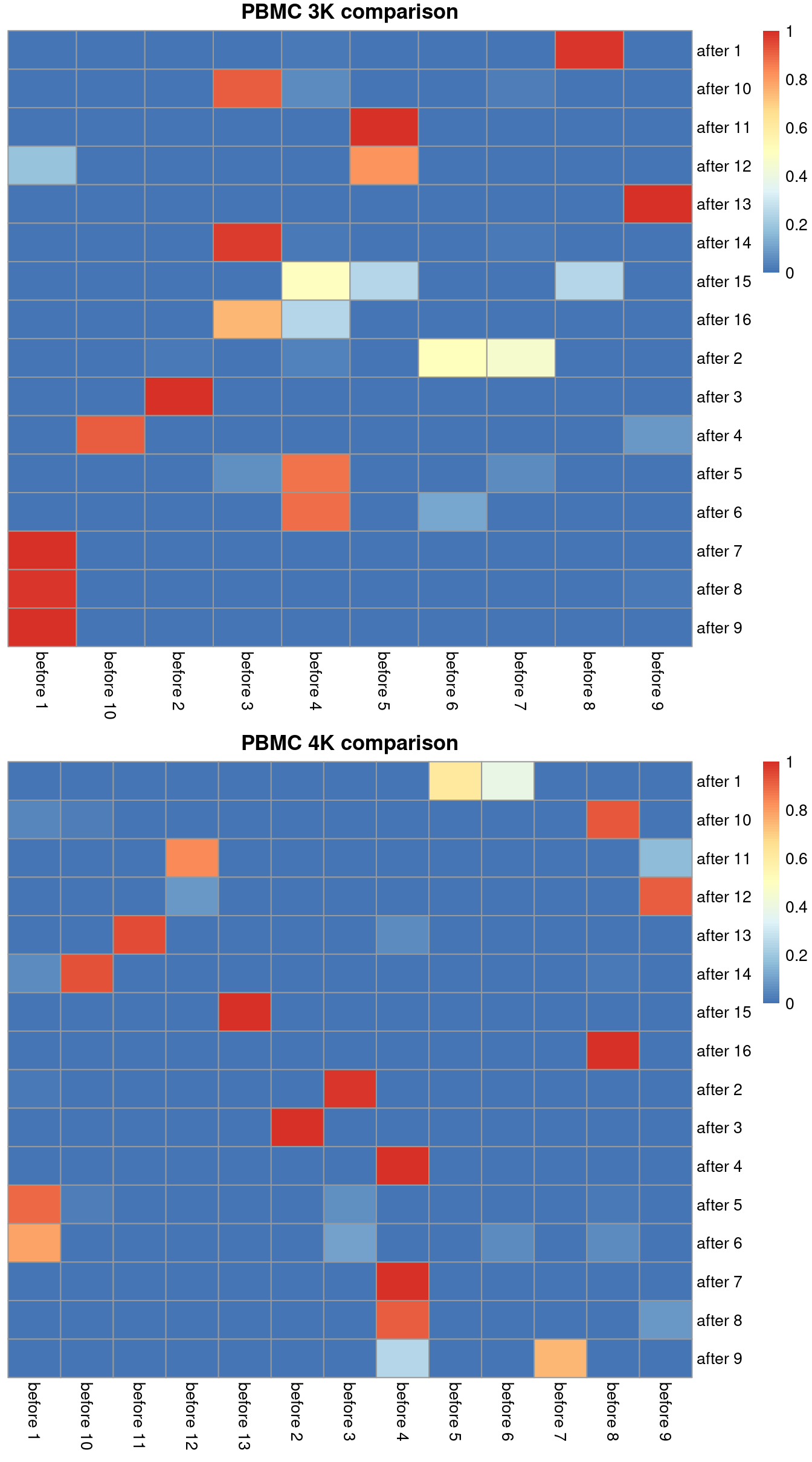
Figure 2.1: Comparison between the clusterings obtained before (columns) and after MNN correction (rows). One heatmap is generated for each of the PBMC 3K and 4K datasets, where each entry is colored according to the proportion of cells distributed along each row (i.e., the row sums equal unity).
We use the adjusted Rand index (Advanced Section 5.3) to quantify the agreement between the clusterings before and after batch correction. Recall that larger indices are more desirable as this indicates that within-batch heterogeneity is preserved, though this must be balanced against the ability of each method to actually perform batch correction.
library(bluster)
ri3k <- pairwiseRand(clusters.mnn[mnn.out$batch==1], colLabels(pbmc3k), mode="index")
ri3k
## [1] 0.7361## [1] 0.8301We can also break down the ARI into per-cluster ratios for more detailed diagnostics (Figure 2.2). For example, we could see low ratios off the diagonal if distinct clusters in the within-batch clustering were incorrectly aggregated in the merged clustering. Conversely, we might see low ratios on the diagonal if the correction inflated or introduced spurious heterogeneity inside a within-batch cluster.
# For the first batch.
tab <- pairwiseRand(colLabels(pbmc3k), clusters.mnn[mnn.out$batch==1])
heat3k <- pheatmap(tab, cluster_row=FALSE, cluster_col=FALSE,
    col=rev(viridis::magma(100)), main="PBMC 3K probabilities", silent=TRUE)

# For the second batch.
tab <- pairwiseRand(colLabels(pbmc4k), clusters.mnn[mnn.out$batch==2])
heat4k <- pheatmap(tab, cluster_row=FALSE, cluster_col=FALSE,
    col=rev(viridis::magma(100)), main="PBMC 4K probabilities", silent=TRUE)

gridExtra::grid.arrange(heat3k[[4]], heat4k[[4]])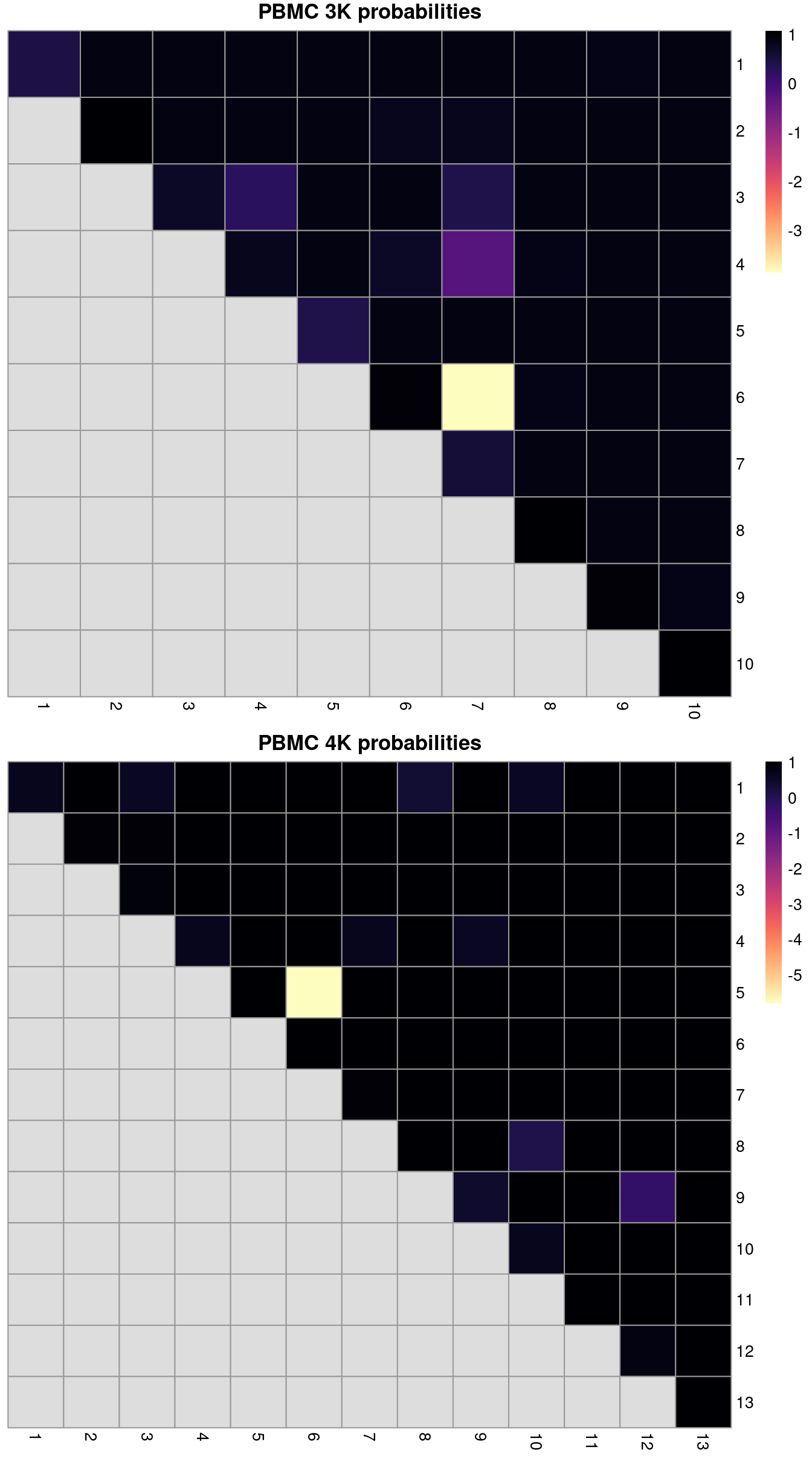
Figure 2.2: ARI-derived ratios for the within-batch clusters after comparison to the merged clusters obtained after MNN correction. One heatmap is generated for each of the PBMC 3K and 4K datasets.
2.4 MNN-specific diagnostics
For fastMNN(), one useful diagnostic is the proportion of variance within each batch that is lost during MNN correction.
Specifically, this refers to the within-batch variance that is removed during orthogonalization with respect to the average correction vector at each merge step.
This is returned via the lost.var field in the metadata of mnn.out, which contains a matrix of the variance lost in each batch (column) at each merge step (row).
##          [,1]     [,2]
## [1,] 0.006617 0.003315
Large proportions of lost variance (>10%) suggest that correction is removing genuine biological heterogeneity. This would occur due to violations of the assumption of orthogonality between the batch effect and the biological subspace (Haghverdi et al. 2018). In this case, the proportion of lost variance is small, indicating that non-orthogonality is not a major concern.
Another MNN-related diagnostic involves examining the variance in the differences in expression between MNN pairs.
A small variance indicates that the correction had little effect - either there was no batch effect, or any batch effect was simply a constant shift across all cells.
On the other hand, a large variance indicates that the correction was highly non-linear, most likely involving subpopulation-specific batch effects.
This computation is achieved using the mnnDeltaVariance() function on the MNN pairings produced by fastMNN().
library(batchelor)
common <- rownames(mnn.out)
vars <- mnnDeltaVariance(pbmc3k[common,], pbmc4k[common,],
   pairs=metadata(mnn.out)$merge.info$pairs)
vars[order(vars$adjusted, decreasing=TRUE),]
## DataFrame with 13431 rows and 4 columns
## mean total trend adjusted
## <numeric> <numeric> <numeric> <numeric>
## ENSG00000111796 0.404086 1.487536 0.657367 0.830169
## ENSG00000257764 0.320638 1.044040 0.548209 0.495831
## ENSG00000170345 2.543318 1.342864 0.948955 0.393909
## ENSG00000187118 0.313542 0.916383 0.538257 0.378126
## ENSG00000177606 1.799190 1.400792 1.033322 0.367470
## ... ... ... ... ...
## ENSG00000204482 0.786304 0.537895 0.97769 -0.439796
## ENSG00000011600 1.176075 0.628421 1.07374 -0.445319
## ENSG00000101439 1.135830 0.626148 1.07300 -0.446850
## ENSG00000158869 0.927395 0.575360 1.03902 -0.463658
## ENSG00000105374 1.219511 0.536416 1.07336 -0.536943Such genes with large variances are particularly interesting as they exhibit complex differences between batches that may reflect real biology. For example, in Figure 2.3, the KLRB1-positive clusters in the second batch lack any counterpart in the first batch, despite the two batches being replicates. This may represent some kind of batch-specific state in two otherwise identical populations, though whether this is biological or technical in nature is open for interpretation.
library(scater)
top <- rownames(vars)[order(vars$adjusted, decreasing=TRUE)[1]]
gridExtra::grid.arrange(
    plotExpression(pbmc3k, x="label", features=top) + ggtitle("3k"),
    plotExpression(pbmc4k, x="label", features=top) + ggtitle("4k"),
    ncol=2
)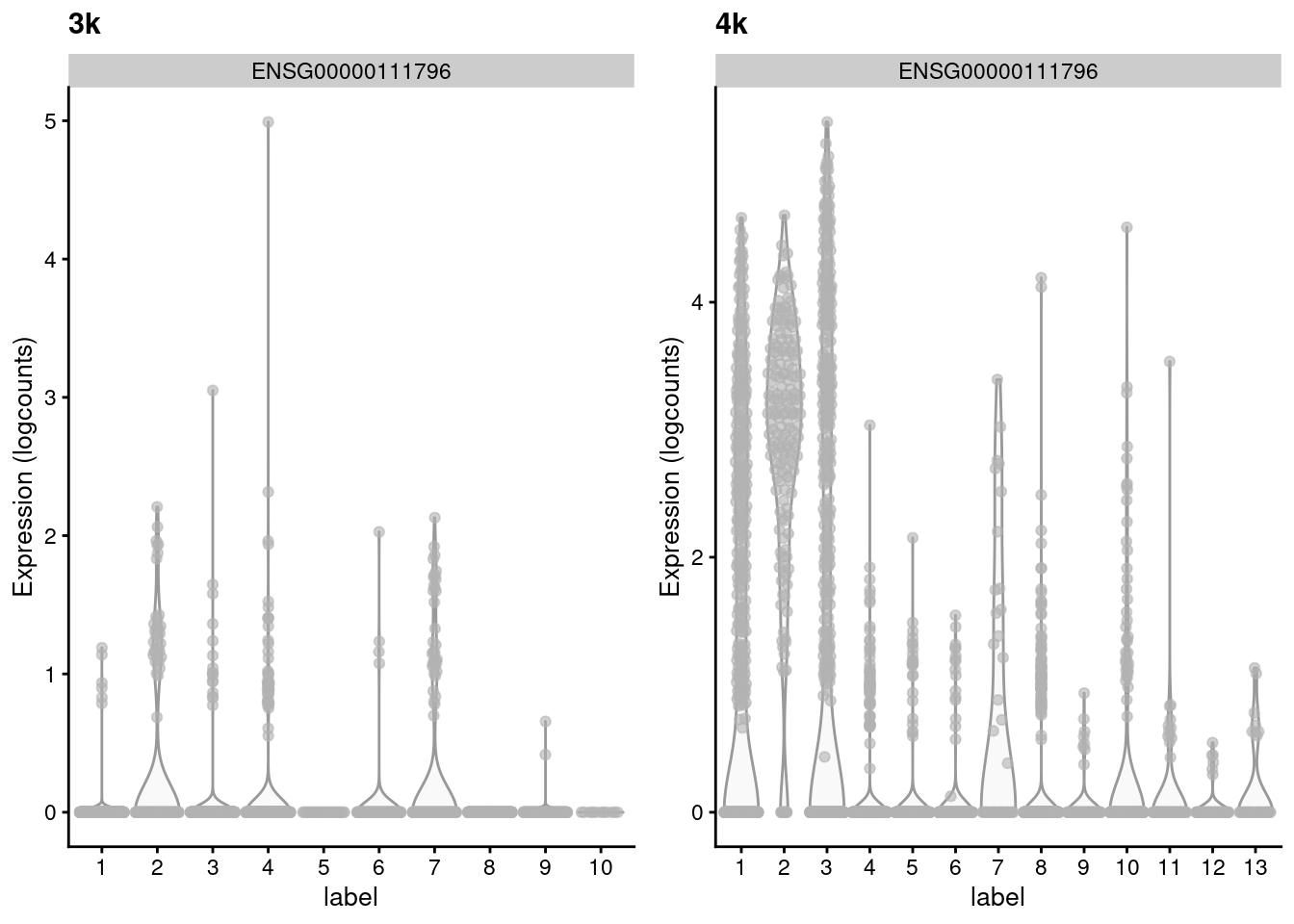
Figure 2.3: Distribution of the expression of the gene with the largest variance of MNN pair differences in each batch of the the PBMC dataset.
Session Info
R version 4.1.0 (2021-05-18)
Platform: x86_64-pc-linux-gnu (64-bit)
Running under: Ubuntu 20.04.2 LTS

Matrix products: default
BLAS:   /home/biocbuild/bbs-3.13-bioc/R/lib/libRblas.so
LAPACK: /home/biocbuild/bbs-3.13-bioc/R/lib/libRlapack.so

locale:
 [1] LC_CTYPE=en_US.UTF-8       LC_NUMERIC=C
 [3] LC_TIME=en_US.UTF-8        LC_COLLATE=C
 [5] LC_MONETARY=en_US.UTF-8    LC_MESSAGES=en_US.UTF-8
 [7] LC_PAPER=en_US.UTF-8       LC_NAME=C
 [9] LC_ADDRESS=C               LC_TELEPHONE=C
[11] LC_MEASUREMENT=en_US.UTF-8 LC_IDENTIFICATION=C

attached base packages:
[1] parallel  stats4    stats     graphics  grDevices utils     datasets
[8] methods   base

other attached packages:
 [1] scater_1.20.0               ggplot2_3.3.3
 [3] scuttle_1.2.0               HDF5Array_1.20.0
 [5] rhdf5_2.36.0                DelayedArray_0.18.0
 [7] Matrix_1.3-3                pheatmap_1.0.12
 [9] bluster_1.2.0               batchelor_1.8.0
[11] BiocSingular_1.8.0          SingleCellExperiment_1.14.0
[13] SummarizedExperiment_1.22.0 Biobase_2.52.0
[15] GenomicRanges_1.44.0        GenomeInfoDb_1.28.0
[17] IRanges_2.26.0              S4Vectors_0.30.0
[19] BiocGenerics_0.38.0         MatrixGenerics_1.4.0
[21] matrixStats_0.58.0          BiocStyle_2.20.0
[23] rebook_1.2.0

loaded via a namespace (and not attached):
 [1] bitops_1.0-7              filelock_1.0.2
 [3] RColorBrewer_1.1-2        tools_4.1.0
 [5] bslib_0.2.5.1             utf8_1.2.1
 [7] R6_2.5.0                  irlba_2.3.3
 [9] ResidualMatrix_1.2.0      vipor_0.4.5
[11] DBI_1.1.1                 colorspace_2.0-1
[13] rhdf5filters_1.4.0        withr_2.4.2
[15] tidyselect_1.1.1          gridExtra_2.3
[17] compiler_4.1.0            graph_1.70.0
[19] BiocNeighbors_1.10.0      labeling_0.4.2
[21] bookdown_0.22             sass_0.4.0
[23] scales_1.1.1              stringr_1.4.0
[25] digest_0.6.27             rmarkdown_2.8
[27] XVector_0.32.0            pkgconfig_2.0.3
[29] htmltools_0.5.1.1         sparseMatrixStats_1.4.0
[31] limma_3.48.0              highr_0.9
[33] rlang_0.4.11              DelayedMatrixStats_1.14.0
[35] farver_2.1.0              generics_0.1.0
[37] jquerylib_0.1.4           jsonlite_1.7.2
[39] BiocParallel_1.26.0       dplyr_1.0.6
[41] RCurl_1.98-1.3            magrittr_2.0.1
[43] GenomeInfoDbData_1.2.6    ggbeeswarm_0.6.0
[45] Rhdf5lib_1.14.0           Rcpp_1.0.6
[47] munsell_0.5.0             fansi_0.4.2
[49] viridis_0.6.1             lifecycle_1.0.0
[51] stringi_1.6.2             yaml_2.2.1
[53] edgeR_3.34.0              zlibbioc_1.38.0
[55] grid_4.1.0                dqrng_0.3.0
[57] crayon_1.4.1              dir.expiry_1.0.0
[59] lattice_0.20-44           cowplot_1.1.1
[61] beachmat_2.8.0            locfit_1.5-9.4
[63] CodeDepends_0.6.5         metapod_1.0.0
[65] knitr_1.33                pillar_1.6.1
[67] igraph_1.2.6              codetools_0.2-18
[69] ScaledMatrix_1.0.0        XML_3.99-0.6
[71] glue_1.4.2                evaluate_0.14
[73] scran_1.20.0              BiocManager_1.30.15
[75] vctrs_0.3.8               purrr_0.3.4
[77] gtable_0.3.0              assertthat_0.2.1
[79] xfun_0.23                 rsvd_1.0.5
[81] viridisLite_0.4.0         tibble_3.1.2
[83] beeswarm_0.3.1            cluster_2.1.2
[85] statmod_1.4.36            ellipsis_0.3.2
References
Büttner, Maren, Zhichao Miao, F Alexander Wolf, Sarah A Teichmann, and Fabian J Theis. 2019. “A Test Metric for Assessing Single-Cell Rna-Seq Batch Correction.” Nature Methods 16 (1): 43–49.
Haghverdi, L., A. T. L. Lun, M. D. Morgan, and J. C. Marioni. 2018. “Batch effects in single-cell RNA-sequencing data are corrected by matching mutual nearest neighbors.” Nat. Biotechnol. 36 (5): 421–27.